
February, 2024
The main goal of regression analysis is to build a model that accurately predicts the target variable based on the input features. However, the accuracy of the model can only be determined by comparing its predicted values to the actual target values.
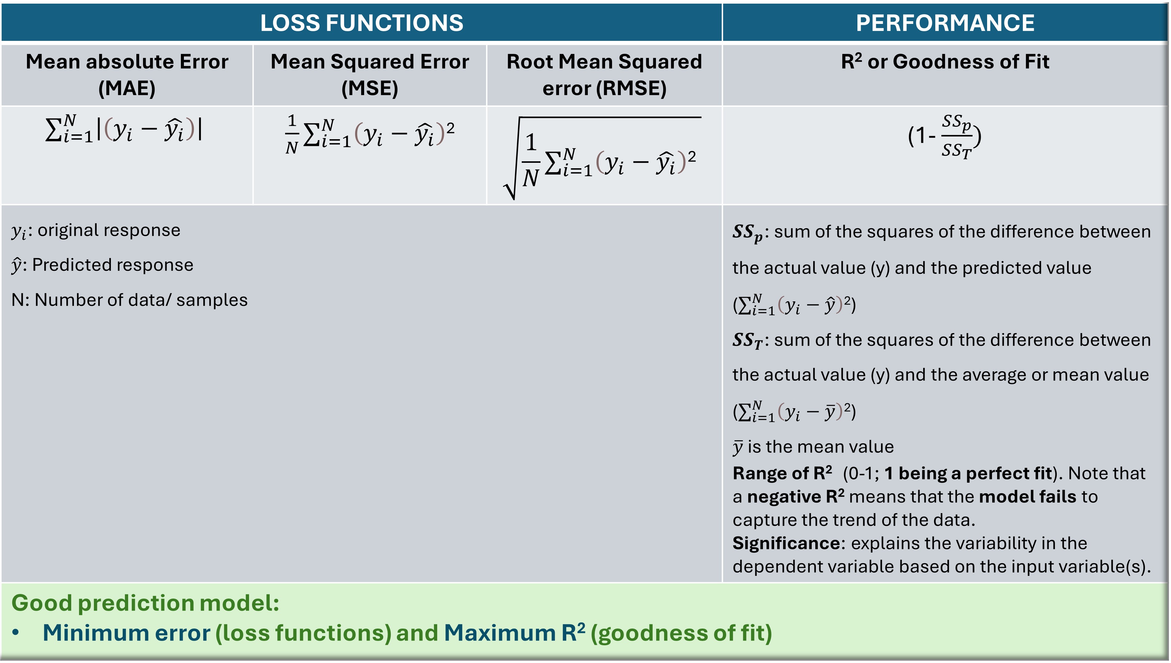
Several evaluation metrics can be used in regression analysis, such as mean squared error (MSE), root mean squared error (RMSE), mean absolute error (MAE), and R2. While MSE, RMSE, and MAE are the error functions, R2, also known as goodness of fit or coefficient of determination, measures the model’s performance. The mathematical equations of these evaluation metrics are tabulated for understanding and convenience.
 The evaluation metrics for regression analysis.
In general, a good regression model should have low values for MSE, RMSE, and MAE, indicating that the predicted values are close to the actual values. A high R2 score indicates that the model can explain a large proportion of the variance in the data.
The choice of metric depends on the specific problem and the desired outcome. That being said, I will demonstrate how the number (quantity) and quality (i.e., how essential they are to the response ) of input features impact the model fitting and prediction, and consequently the evaluation metrics in two separate tutorials.
A brief technical note on the working dataset
The dataset comprises 204 thermoelectric materials (compositions), their room temperature transport properties, and the performance metrics, ZT.
Note that two features (S2 and sigma/kappa) are derived, and they play a major role in the evaluation of ZT.
ZT is directly proportional to S2, sigma (σ), and holds an inverse relationship with kappa (κ). Here is the equation connecting ZT with the transport properties.

Let’s now go through the coding steps to compute the error functions and performance metrics.
Coding for Computing Error/Loss functions and performance metric
Step 1: Importing the relevant libraries and loading the dataset
import numpy as np
import matplotlib.pyplot as plt
import pandas as pd

# for machine learning
from sklearn.model_selection import train_test_split
from sklearn.linear_model import LinearRegression
from sklearn.preprocessing import PolynomialFeatures

# for loss functions and R square
from sklearn.metrics import mean_absolute_error
from sklearn.metrics import mean_squared_error
from  sklearn.metrics import r2_score
Input feature considered: kappa; Target: ZT
dataset = pd.read_csv('RT_TEprop.csv')
X = dataset.iloc[:, 4].values
y = dataset.iloc[:, -1].values
Step 2: Splitting data into training and test sets
X_train, X_test, y_train, y_test = train_test_split(X, y, test_size = 0.1, random_state = 0)# Reshaping required as fit() method of the LinearRegression class expects a 2D array as input.
X_train=X_train.reshape(183,1)
y_train=y_train.reshape(183,1)Step 3: Fitting linear regression model to the training set
lr = LinearRegression()
lr.fit(X_train, y_train)
Step 4: Prediction
X_test=X_test.reshape(21,1)
y_test=y_test.reshape(21,1)
y_pred = lr.predict(X_test)
np.set_printoptions(precision=2)
print(np.concatenate((y_pred.reshape(len(y_pred),1), y_test.reshape(len(y_test),1)),1))
Plotting
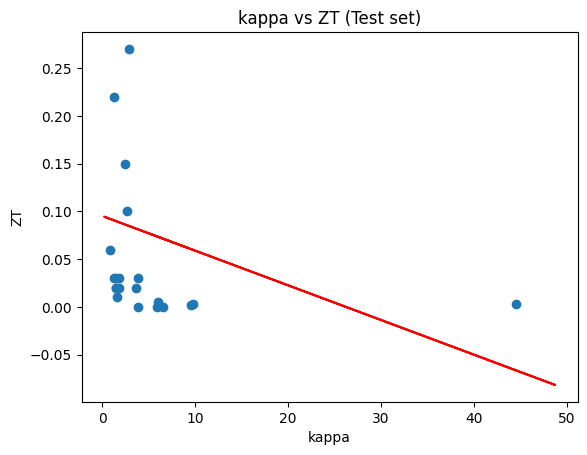
plt.scatter(X_test, y_test)
plt.plot(X_train, lr.predict(X_train), "r")
plt.title("kappa vs ZT (Test set)")
plt.xlabel("kappa")
plt.ylabel("ZT")
plt.show()
Step 5: Computing error/ loss functions such as MAE, MSE, RMSE
print("MAE",mean_absolute_error(y_test,y_pred))
MAE 0.07059993216927259
print("Mean square error is ",mean_squared_error(y_test,y_pred))
Mean square error is 0.00606286753428833
rmse_lr = np.sqrt(mean_squared_error(y_test, y_pred))
rmse_lr
0.07786441763917798
Step 6: Computing R2
r2_score_lr= r2_score(y_test, y_pred)
r2_score_lr
-0.1281233534684132
A negative goodness of fit in machine learning suggests that the model performs worse than a simple baseline model. This indicates that the model needs improvement or a different modeling approach to better capture the underlying patterns in the data.
Therefore, we can apply polynomial regression fitting to see if there is any improvement in the model's performance.
We now fit a polynomial regression model to the training dataset using the same input variable, kappa to observe any improvement in the R2 value. We will be using the same dataset as before. So, let's directly move to the polynomial regression part.
Import PolynomialFeatures from sklearn.preprocessing class for polynomial regression fitting. 'PolynomialFeatures' generates a new feature matrix of polynomial combinations with specified degrees followed by applying the fit_tranform() method to the input variable.
 poly = PolynomialFeatures(degree=2)
poly_features_1 = poly.fit_transform(X.reshape(-1,1))
X1_train, X1_test, y1_train, y1test = train_test_split(poly_features_1, y, test_size=0.1, random_state=42)poly_features_1.shapeNote: New matrix has 204 rows, 3 columns for kappa values. Original data: 204 rows, 1 column.

poly_features_1A snapshot of the output, displayig the new matrix, is shown below.
array([[1.00e+00, 2.51e+00, 6.32e+00],
       [1.00e+00, 2.27e+00, 5.14e+00],
       [1.00e+00, 2.50e+00, 6.25e+00],
       [1.00e+00, 1.79e+00, 3.19e+00],
       [1.00e+00, 2.85e+00, 8.12e+00],
       [1.00e+00, 1.48e+00, 2.20e+00],
       [1.00e+00, 2.17e+00, 4.71e+00],
       [1.00e+00, 1.64e+00, 2.68e+00],
       [1.00e+00, 2.14e+00, 4.60e+00],
       [1.00e+00, 1.49e+00, 2.22e+00],
       [1.00e+00, 1.79e+00, 3.21e+00],
       [1.00e+00, 3.56e+00, 1.27e+01],
Splitting the data into training and test sets
The training dataset consists of 183 rows and 3 columns against 1 column in the original dataset used for simple regression analysis.
X1_train, X1_test, y1_train, y1test = train_test_split(poly_features_1, y, test_size=0.1, random_state=42)
After splitting the data, same steps are followed as before such as linear regression fitting of the training data, prediction using the test set followed by computation of loss functions and R2. The values of these parameters are tabulated with the help of tabulate function of Python tabulate module.
The coding and the output for the same are shown below.
from tabulate import tabulate

Eval_table = [["MAE", 0.089], ["MSE",0.016], ['RMSE', 0.125], ['R-squared', -0.015]]
print(tabulate(Eval_table))
--------- ------
MAE 0.089
MSE 0.016
RMSE 0.125
R-squared -0.015
--------- ------We found that both simple and polynomial linear regression fittings result in similar outcomes with respect to loss functions and R2.
In the next tutorial, we will delve into the impact of incorporating additional input variables and selecting appropriate types of input variables on the evaluation metrics of the machine learning model, aiming for improved prediction outcomes.
Link to the entire code and dataset.