Microstructure Analysis: Comparison of Image Filters for Edge Detection
by Joyita Bhattacharya
Measurement and identification of particle size and morphology from the microstructure of materials play an essential role in determining materials' properties. A precise measurement of these parameters involves resolving the edges/ boundaries of particles from the captured images, also known as microstructure. Thanks to different image processing tools, the task is more straightforward for crisp images. However, the complexity of such analysis becomes more challenging with blurred or distorted images. Let us evaluate the outcome of edge detection on a blurry image subjected to different image processing filters. Here, blurry microstructure implies no sharp gradient between objects (features) and matrix (background); instead, it seems diffuse.
Hence, we aim to identify the right edges of the features.
First, we will apply standard edge-identifying filters such as Sobel, Roberts, and Canny and a sharpening image function (unsharp masking) from the scikit-image.
I will display the python codes and the corresponding output for the above activity stepwise.
Step 1: Import the relevant Python libraries
import numpy as np
import matplotlib.pyplot as plt
from skimage import io, color
from skimage.filters import difference_of_gaussians, window
from scipy.fft import fftn, fftshift
from skimage import filters
from skimage.filters import sobel,sobel_v, sobel_h, roberts
from skimage.feature import canny
Step 2: Load the image (microstructure)
im = io.imread('im1_blur.jpg')
plt.imshow(im, cmap = 'gray')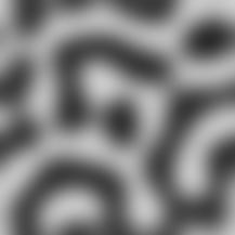 Defocussed microstructure (simulated)
Step 3: Apply the different filter operators on the image matrix and compare their outputs
We will be comparing different filters for edge detection in this defocussed image. Let us try to sharpen the features of the image using unsharp masking filter of scikit-image.
Unsharp Masking filter
Sharpimg = filters.unsharp_mask(im, radius = 50.0, amount = 1.0)
plt.imshow(Sharpimg, cmap ='gray')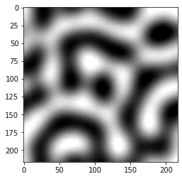 Unsharp masking filtered image
 Sobel filter
im1_sobel = sobel(im)
plt.imshow(im1_sobel, cmap='gray')
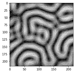 Image after applying Sobel filter
 Roberts filter
im1_roberts = roberts(im)
plt.imshow(im1_roberts, cmap='gray')
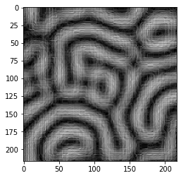 Image after applying Roberts filter
 Canny filter
im1_canny= canny(im)
plt.imshow(im1_canny, cmap ='gray')
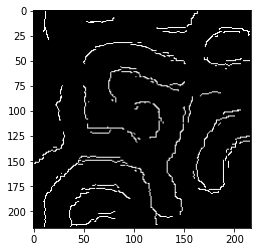 Image after applying Canny filter
 Fourier Transform of the Image
Please read my blog on Fourier Transform to understand the coding steps.
- ✓ We first apply the Fast Fourier Transform (fft) on the image followed by fftshift function to bring back the origin of the spectrum to the center which is otherwise off-centered' and located on the top leftmost corner of the fft spectrum.
im1_F = np.fft.fft2(im)
im1_F_02 = np.fft.fftshift(im1_F)
plt.imshow(np.log(abs(im1_F_02)), cmap ='gray')
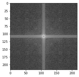 Spectrum in Fourier space after shifting the origin to the center
 - ✓Generate a high frquency mask to allow high frequency components to detect edges. Block the center with the mask
mask_h = np.ones((nx,ny), np.uint8) # mask should have the same dimension as that of the image
center_x = nx/2
center_y = ny/2

# OPEN GRID
x, y = np.ogrid[:nx, :ny]
circle_mask = (x-center_x)**2 + (y-center_y)**2 <= 2.5**2
mask_h[circle_mask] = 0
plt.imshow(mask_h, cmap ='gray')
im1_F_02_c= im1_F_02.copy()

#black out the center by applying high frequency mask
im1_F_02_h = im1_F_02_c* mask_h

#show the image
plt.imshow(abs(im1_F_02_h), cmap ='gray')
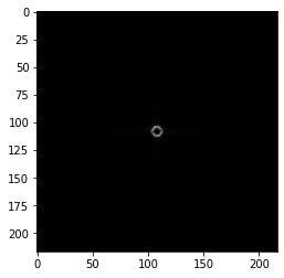 Masked Spectrum
 - ✓Shifting the origin back to its original location using ifftshift function of NumPy followed by inverse Fourier Transform to retrieve the original image.
im1_F_02_originBack = np.fft.ifftshift(im1_F_02_h)
originalImage = np.fft.ifft2(im1_F_02_originBack)
plt.imshow(np.log(abs(originalImage)), cmap ='gray')
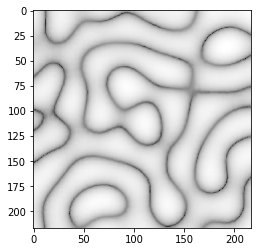 Image after Fourier Transform
 Comparison of different image filters for edge detection
fig, ax = plt.subplots(1, 5, figsize =(15,15))

ax[0].imshow(im, cmap ='gray')
ax[0].set_title("original", fontsize = 10)
ax[1].imshow(np.log(abs(originalImage)), cmap ='gray')
ax[1].set_title("Fourier Transformed", fontsize = 10)
ax[2].imshow(im1_sobel, cmap ='gray')
ax[2].set_title("Sobel filter", fontsize = 10)
ax[3].imshow(im1_roberts, cmap ='gray')
ax[3].set_title("Roberts filter", fontsize = 10)
ax[4].imshow(im1_canny, cmap ='gray')
ax[4].set_title("Canny filter", fontsize = 10)
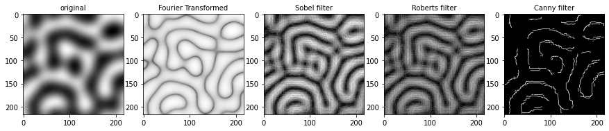 Comparison: Filtered Image
Fourier transformed image shows sharper edges compared to other filtered images.
Click here to view the entire code on Github.