by Joyita Bhattacharya
The usage of different types of devices is an integral part of our everyday life. And these devices are made of myriad combinations of elements forming materials for daily applications. Materials scientists are engaged with the processing of these materials and studying their structures and properties. For example, to develop a new semiconductor, a materials scientist requires to choose the most optimized combination of ingredients from the palette of elements in the Periodic table so that the new semiconductor has the right set of properties.
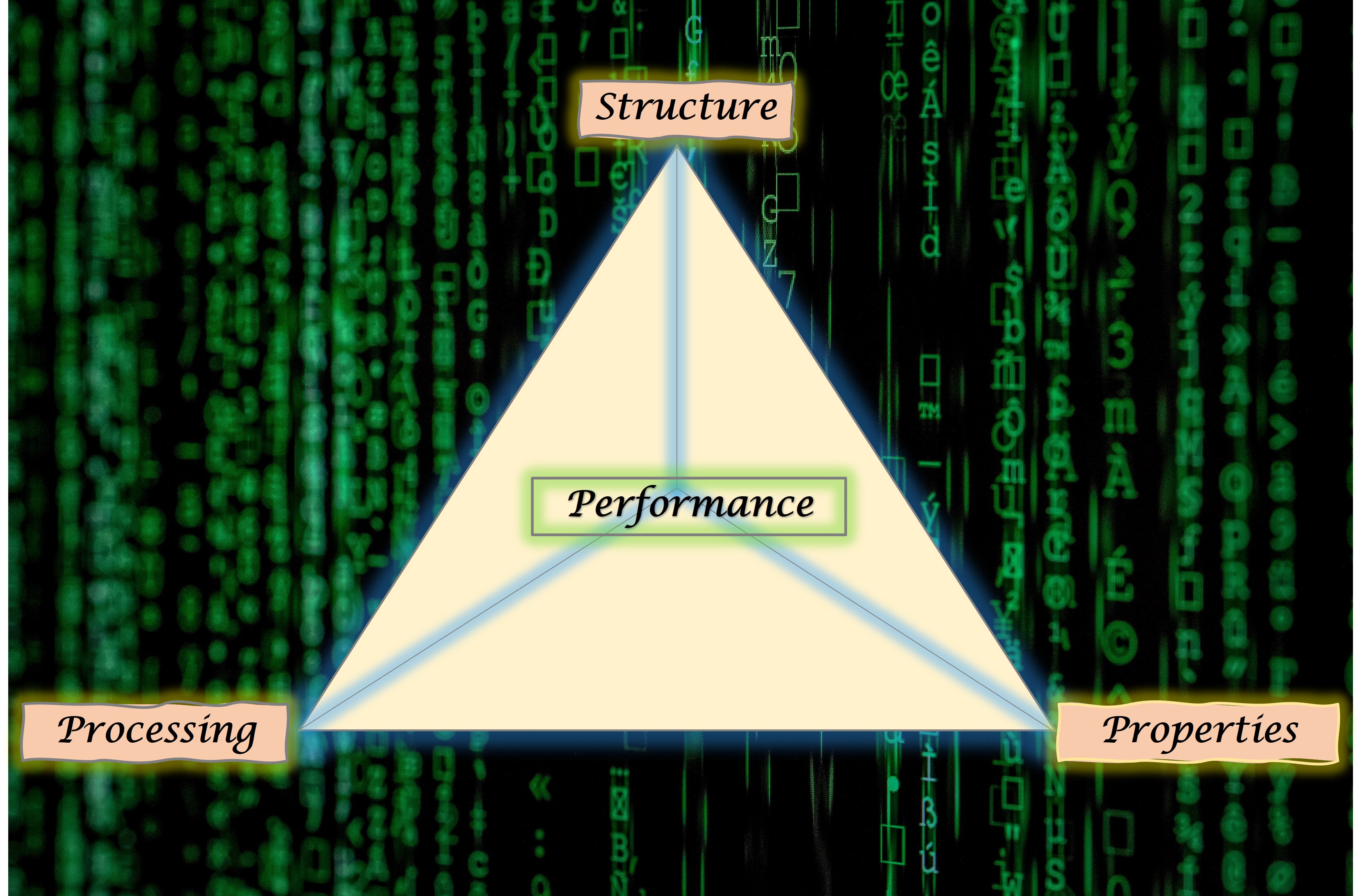
Moreover, performance of a material depends on the trinity of Processing conditions, Structure that spans from electronic scale to macro-scale, and its various structural and functional Properties . Thus, materials scientists have come up with the concept of 'Materials Tetrahedron' where the vertices represent Processing, Structure, Properties and Performance, and the lines connecting these vertices denote interrelations between them. These interconnections are also termed as PSPP linkages.
A comprehensive library of discovered materials with their PSPP linkages will immensely benefit the materials scientists and engineers who aim to design the next super materials such as a battery more efficient than the existing lithium ion battery or a car lighter and stronger than the new Tesla cars.
Hence, extracting meaningful data from these interconnected parameters becomes a crucial step in the design and discovery of high-performance cutting edge materials. The number of parameters can be so diverse that it becomes difficult to extract physics-based cause-effect relations between all these parameters. In such cases, machine learning (ML) can facilitate the development of new knowledge by extracting useful correlations between these parameters.
The very first and crucial step of ML, regardless of the algorithm used, is importing and preprocessing data. Clean data increase the reliability of training and building a machine learning model for successful deployment. This data is further categorized into input variables (also known as predictors/ descriptors in ML language) and outcome (known as target/ response).
Materials data comprise a wide spectrum of descriptors. These include
The target or the response is usually the property dictating the overall performance of the material.
Mining important features from a given dataset is the most critical and challenging step for developing a robust data-driven model. Otherwise, the model will follow the GIGO (Garbage-In-Garbage-Out) rule.
We can show the importance of featurization in materials datasets using a very simple example. Let us consider a dataset containing chemical formulae of several materials and their densities. A chemical formula is represented by a combination of elements and their atomic proportions. For example, the chemical formula (AiBjCkDl) contains four elements A, B, C and D where their corresponding subscripts i, j, k and l represent the number of atoms of each element. For instance, the formula of water is H2O which implies 2 atoms of hydrogen (H is the element symbol) and 1 atom of oxygen (denoted by the symbol O).
Now, to understand the correlations between features and design a super-dense material from such data, we need to unearth the contribution of each element on density. These individual elemental contributions become features (descriptors) for the prediction of the target variable-density in this example. Hence, it is required to split the formula into its individual constituents (or elements) along with their corresponding amount. There is no direct way to achieve this task in the conventional ML technique such as encoding. However, thanks to the Python-based materials libraries, Pymatgen and Matminer, which helps in reaching this goal.
In this article, I will demonstrate how to import constituent elements and their amount from formulae with the aid of the mentioned materials libraries.
Tabulating the descriptor and target variables in comma-delimited (csv) or Excel file (XLSX) is a good way to organize data for machine learning. Once csv/ excel file is ready, we can import the same to any machine learning environment. Here, I will show all the steps, written and run, in Jupyter Notebook. You can also choose Google Colab Notebook for the same purpose.
Step 1: Importing libraries
The first and foremost step is to import all the required basic libraries such as Pandas, NumPy, Matplotlib. Moreover, exclusive libraries for materials data mining (Matminer) and materials analysis (Pymatgen) are installed and then the necessary modules are imported. Both Matminer and Pymatgen are open-source python libraries.
import numpy as np
import pandas as pd
from matplotlib import pyplot as plt
from matplotlib.pyplot import figure
Step 2: Loading data
(Dataset used in here is a subset of the original dataset.)
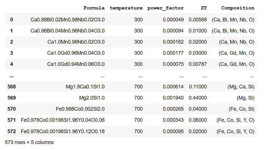
After importing the basic libraries, we need to load and read the csv or excel file containing data using pandas from their file path. In the code snippet below, the first three columns are descriptor variables designated as X, while the last column is the target variable denoted as y.
ds_PF_ZT = pd.read_csv('TE/csv/PF_ZT.csv')
X = ds_PF_ZT.iloc[:, 0:3]
y = ds_PF_ZT.iloc[:, -1]
ds_PF_ZT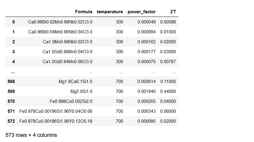
Now, we need to add the individual elements comprising the materials (denoted as Formula in the above Dataframe) as predictors. The synergistic effect of these elemental contributions along with other variables result in the outcome or the response. Here comes the application of Pymatgen and Matminer tools which have featurizers such as core.composition and featurizers.composition to split a given formula into its individual elements. Before proceeding with the coding activity, let me give a preface about Matminer and Pymatgen.
Pymatgen and Matminer: Beneficial libraries for materials data preprocessing
Both Pymatgen and Matminer are open-source Python libraries employed for materials data mining and analysis.
Pymatgen has many modules and sub modules and their respective classes aiding in analysis of structural and functional characteristics of materials. We will be viewing the application of one such module: pymatgen.core.composition and its class: Composition. This class maps each composition in a dataset into individual element and its amount in immutable and hashable form and not as Python dictionary. In Python, there are two types of data: Mutable and Immutable. The values of mutable data can be altered/ mutated while that of immutable cannot. Few examples of mutable data are lists, dictionaries. On the other hand, a tuple is a quintessential example of immutable data. All immutable objects are hashable which means that these objects have unique identification number for easy tracking.
Matminer helps in extracting complex materials attributes applying various featurizers. There are almost more than 70 featurizers (matminer.featurizers) that convert materials attributes into numerical descriptors or vectors. We will focus on Composition featurizer and its ElementFraction class to preprocess our dataset. The said class calculates element fraction of individual elements in a composition.
Step 3: Installing Pymatgen and Matminer
pip install pymatgen
pip install matminer
Note: Matminer and Pymatgen requires Python version 3.6+.
Step 4: Mapping elements and their amount using PymatgenComposition class of pymatgen splits each and every formula, in the given dataset, into constituent elements and their amount. Let's take the first formula, Ca0.98Bi0.02Mn0.98Nb0.02O3.0, in column 1, row 1 :

from pymatgen.core.composition import Composition
ds_PF_ZT['Formula']
Comp = []
for value in ds_PF_ZT['Formula']:
  Comp.append(Composition(value))
  Comp
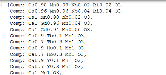
An additional composition column is added to the original dataset containing only the constituent elements corresponding to each composition.
ds_PF_ZT['Composition'] = Comp
ds_PF_ZT
Step 5: Calculation of atomic fraction using ElementFraction class
We now need to add the individual element along with its atomic fraction in the Dataframe to be subjected to machine learning. A class in matminer.featurizers.composition named 'ElementFraction' serves the said intent.
from matminer.featurizers.composition import ElementFraction
ef = ElementFraction()
We, then, create a Dataframe using the featurize_dataframe function which contains all the elements of the periodic table along with other variables. The dimension of the dataframe increased to 573 X 108 (encircled by orange in the output of the code snippet shown below).
ds_PF_ZT = ef.featurize_dataframe(ds_PF_ZT,'Composition')
ds_PF_ZT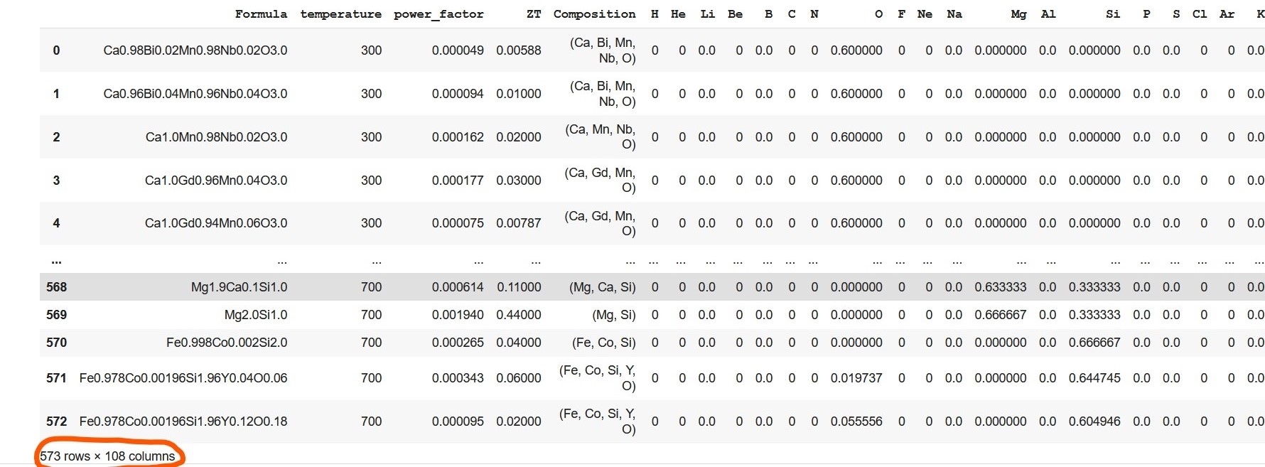
Let me elaborate on element fraction calculation. Let's consider the very first composition (in the formula column of the given dataset). The composition,Ca0.98Bi0.02Mn0.98Nb0.02O3.0, has five elements: Ca (calcium), Bi (bismuth), Mn (manganese), Nb (niobium), and O (oxygen). The amount of Ca present in the formula is 0.98, and the element fraction of Ca is calculated by taking into account the amount of other elements present in the formula. Hence, element fraction of Ca is 0.196 [(0.98)/(0.98+0.02+0.98+0.02+3.0)]. Similarly, element fractions of Bi, Mn, Nb, and O are 0.004, 0.196, 0.004, and 0.6 respectively. The element fraction of the rest of the elements, for this formula, in the periodic table remains zero.
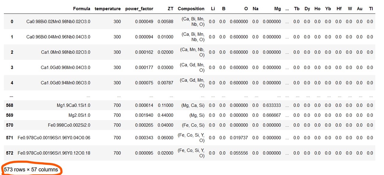
Step 6: Reduction in Dimensionality and display of final, clean, preprocessed data

Note that above Dataframe contains many columns with only zero value. This is due to the non-existence of such elements in compositions in the given dataset. Hence, these zero columns are omitted from the Dataframe which resulted in dimensionality reduction of the Dataframe from 573 rows x 108 columns to 573 rows x 57 columns..
ds_PF_ZT = ds_PF_ZT.loc[:, (ds_PF_ZT != 0).any(axis=0)]
ds_PF_ZT
The above preprocessed, clean Dataframe is the final form ready for machine learning. It is a good practice to keep the response or target column as the last one in the final Dataframe.
The code is published on Github.
Concluding RemarksIn the contemporary world, 'data is the new oil'-a phrase coined by a British mathematician Clive Humby. Hence, mining this treasure to get maximum useful latent information is necessary for technological advancement. From a materials science perspective, numerous materials attributes, processing parameters, and elemental contributions form a complete dataset. These details constitute a part of materials informatics which play an enormous role in the discovery of new high-performance materials. Uncovering the role of constituent elements on material properties is a crucial but tricky job. Matminer and Pymatgen have made this task easier. Here I described the usage of a few relevant modules of these materials libraries to gather elemental information from the original dataset. I hope this article is informative, especially for engineers and scientists working on the design and discovery of new materials.
Please feel free to connect if you need any clarifications and do share your feedback and suggestions.
Thank you for reading!