How to Apply Binary Logistic Regression Analysis for Prediction of Materials Properties

March, 2024

---

In this tutorial, I will demonstrate how logistic regression analysis through machine learning can be instrumental in qualitatively predicting the properties of materials. The term 'qualitatively' indicates that the target or output variable is categorical. For instance, whether a given material (composition) is exhibiting a certain property or not. The output of binary logistic regression is binary/ dichotomous, offering only two possible results, such as yes or no, true or false, success or failure.

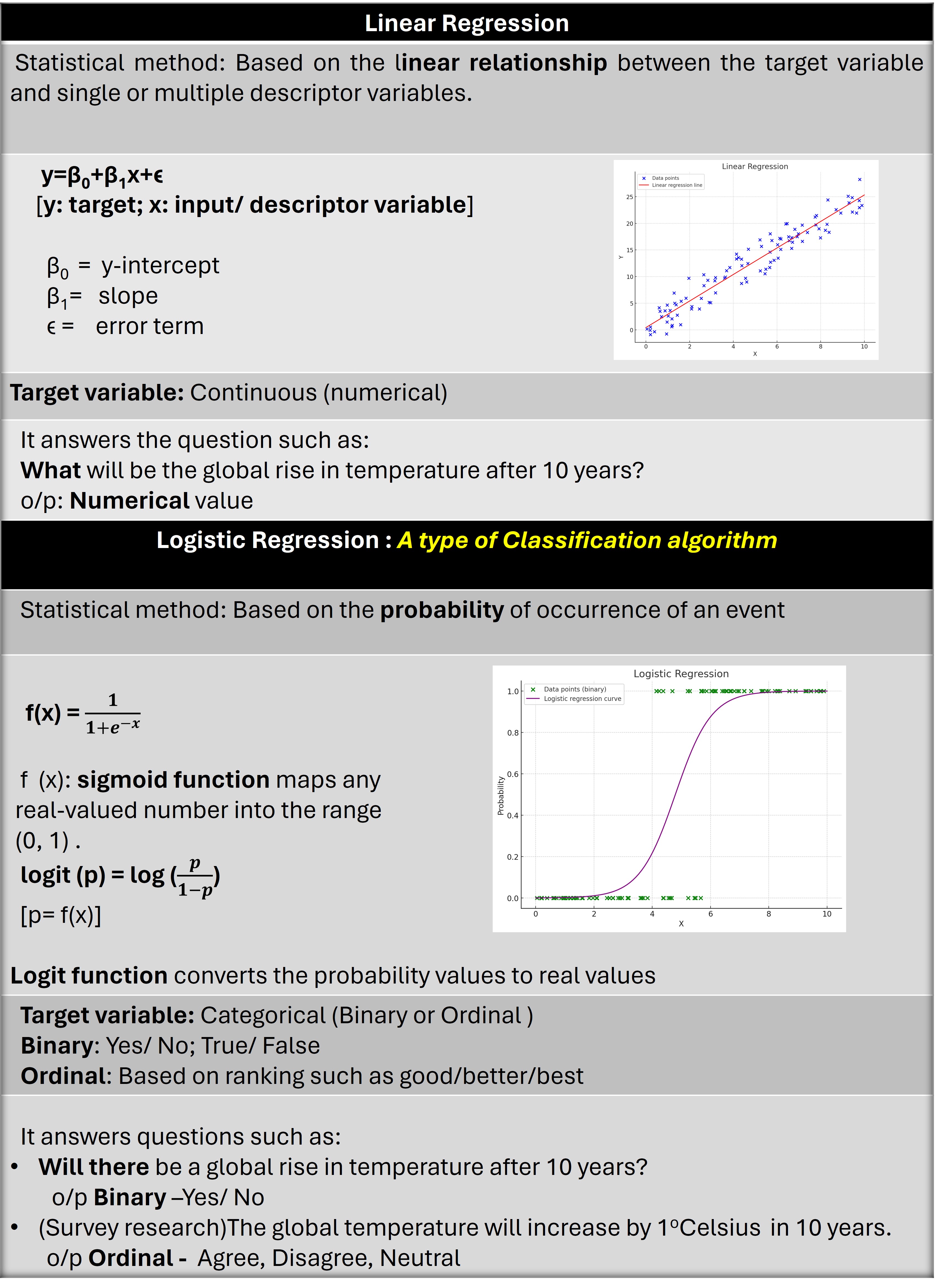
Here is a quick overview of linear regression and logistic regression in tabular form. This will help to understand the coding steps shown in the next section.

Click this link for further reading on logistic regression.

The Coding

Dataset: I have generated a hypothetical dataset comprising 150 unique compositions (materials) alongside their respective corrosion rates, density currents, polarization resistance, and corrosion resistance. The dataset encompasses a broad spectrum of metals, alloys, and composites, each assigned fictional corrosion-related properties to simulate diverse corrosion behaviors in different media.

Aim: To predict corrosion behaviour of materials qualitatively using machine learning and applying binary logistic regression.

Task 1: Import necessary Python libraries

import numpy as np
import matplotlib.pyplot as plt
import pandas as pd
from sklearn.model_selection import train_test_split
from sklearn.linear_model import LogisticRegression
from sklearn.metrics import confusion_matrix, accuracy_score 

Task 2: Load Dataset, Define X, y.

data = pd.read_csv('SyntheticCorrData3.csv', encoding='latin') 

# Create a DataFrame
df = pd.DataFrame(data)

Below is the screenshot of the dataset.

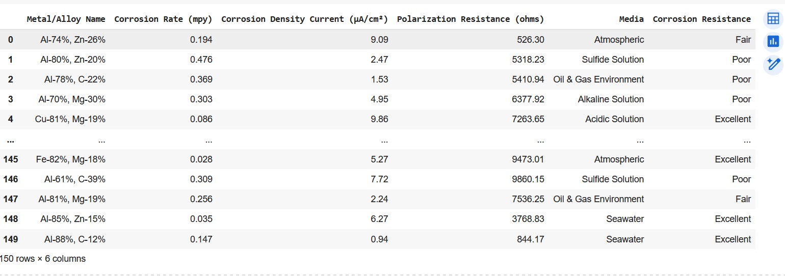Screenshot of the dataframe showing corrosion properties of materials

The aim of this activity is to learn binary logistic regression. Hence we will choose only those rows containing 'poor' and 'excellent' as target/ output. The code to make the refined dataset with the said targets is shown below.

 # filtering the rows with 'poor' and 'excellent' corrosion resistance 
df_binary = df[df['Corrosion Resistance'].str.contains('Poor|Excellent')]

Output

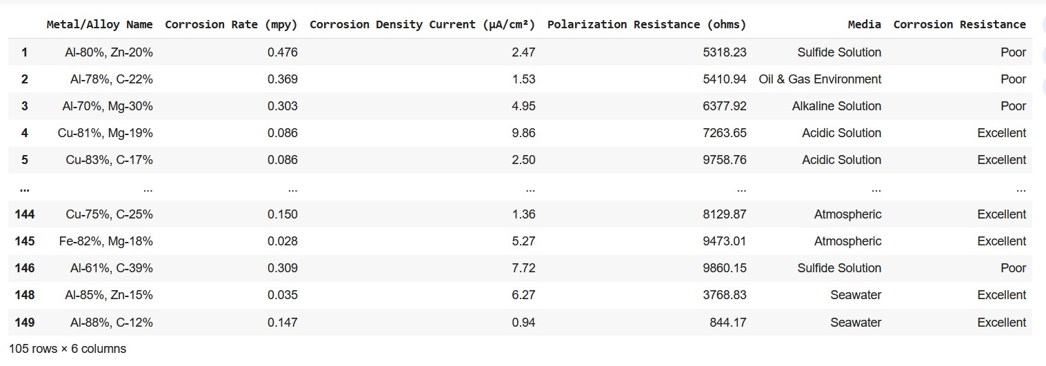Screenshot of the dataframe showing corrosion resistance 'poor' and 'excellent'.

Let me now define the input features and the output/ target variable.

4 Input variables (Xs): Corrosion rate, Corrosion density current, Polarization resistance, Media. Note that three input variables have numerical data and variable 'Media' has categorial data.

Target (y): Corrosion Resistance (categorical data)

X = df.iloc[:, 1:5].values
y = df.iloc[:, -1].values

Task 3: Encoding Categorical Data

Input variables have both numeric and categorical data. Iconverted the categorical data to numeric by encoding by using label encoder from sklearn.preprocessing.

from sklearn.preprocessing import LabelEncoder
le = LabelEncoder()
df['Media'] = le.fit_transform(df['Media'])

Each label or category in 'Media' variable is now designated by a number. Run the below code to check the labels and their corresponding number.

list(le.inverse_transform([0,1,2,3,4,5]))

Output

['Acidic Solution', 'Alkaline Solution',
 'Atmospheric', 'Oil & Gas Environment', 'Seawater', 'Sulfide Solution']

Similarly, the categorical target variable is also encoded with label encoder.

df_binary['Corrosion Resistance'] = le.fit_transform(y)
y=df_binary['Corrosion Resistance']

list(le.classes_)

The encoded output are 0 and 1 representing 'Excellent' and 'Poor' respectively.

 list(le.inverse_transform([0,1]))

Output

 ['Excellent', 'Poor']

Task 4: Training the data: Splitting it into Training set and Test set (90:10)

X_train, X_test, y_train, y_test = train_test_split(X, y, test_size = 0.1, random_state = 0)

Task 5: Fitting data with Logistic Regression Model

classifier = LogisticRegression(random_state = 0)
classifier.fit(X_train, y_train)

Task 6: Prediction with test set

y_pred = classifier.predict(X_test)

Task 7: Checking the performance of the model with Confusion Matrix

A confusion matrix in machine learning is a table that visualizes the performance of a classification algorithm. It compares the predicted classes of a model with the actual classes from the dataset (see the graphical representation below).

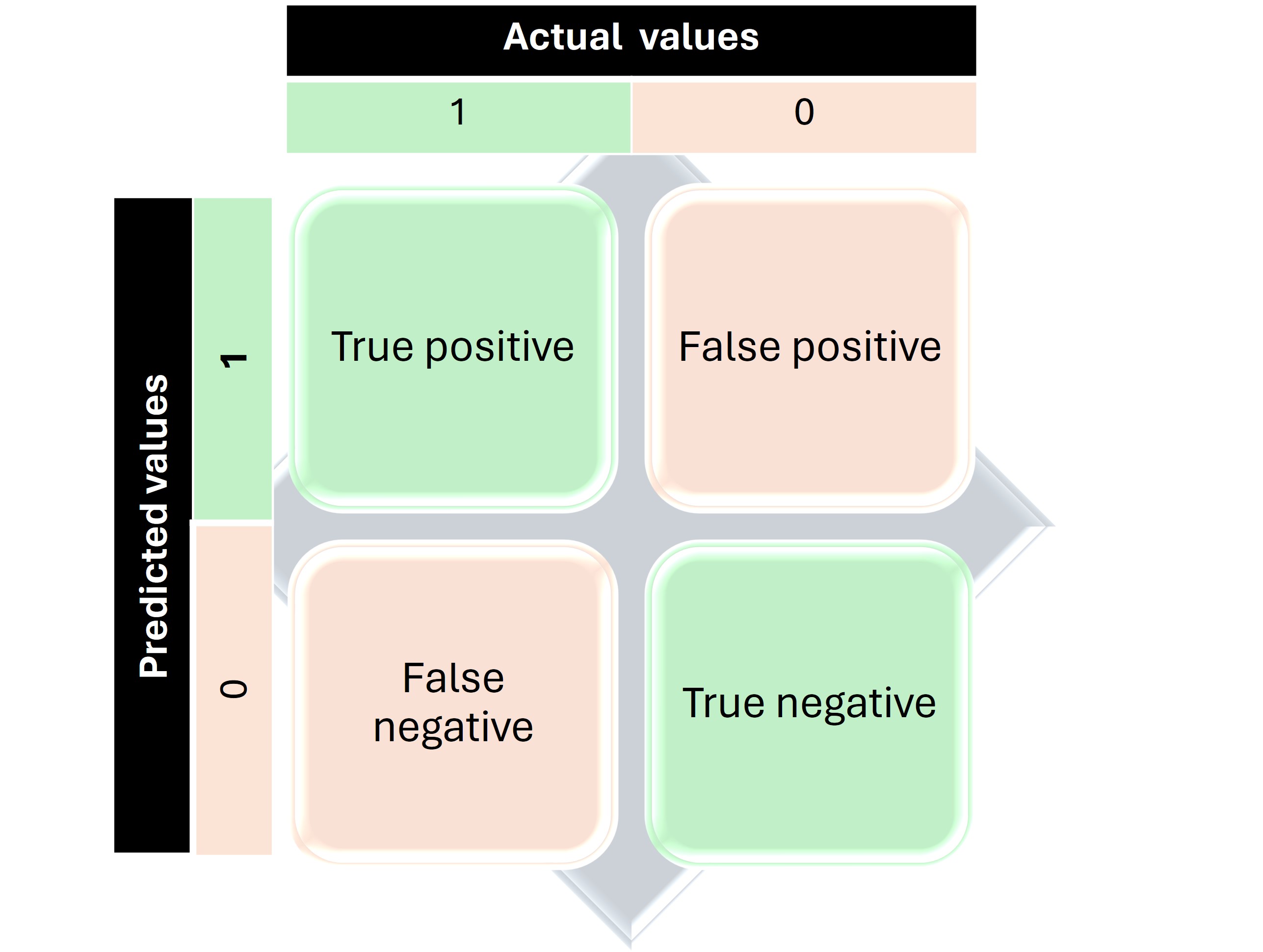Graphical representation of Confusion Matrix.

cm = confusion_matrix(y_test, y_pred)
print(cm)
accuracy_score(y_test, y_pred)

Output

[[6 0]
 [0 5]]
 1.0 

Task 8: Visual representation of the performance of the model with Seaborn

import seaborn as sns
sns.heatmap(cm, annot=True)

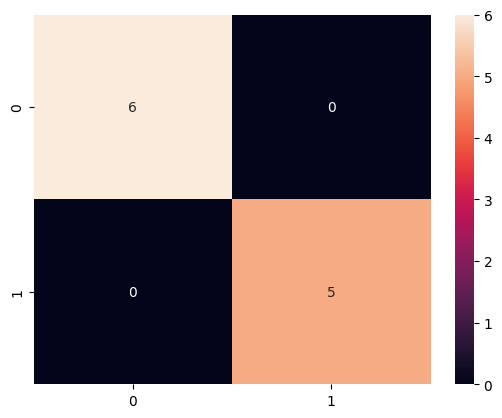Confusion matrix

Representation in percentage

sns.heatmap(cm/np.sum(cm), annot=True,
            fmt='.2%', cmap='GnBu')

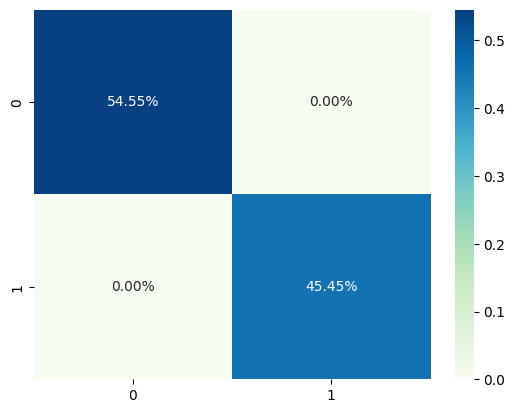Confusion matrix in percentage.

Click to view the entire code.

In this guide, I demonstrated how to perform binary logistic regression by focusing exclusively on two categories (poor and excellent) of corrosion resistance behavior from the initial dataset.

Nonetheless, it's possible to train the complete dataset that includes multiple categorical outcomes using logistic regression. For such scenarios, ordinal logistic regression paired with an ordinal encoder is required.

Stay tuned for my upcoming tutorial on coding with ordinal regression in detail!