

by Joyita Bhattacharya | posted on June 14, 2023
Aim of the tutorial: To demonstrate the coding steps for microstructure (image) classification using Convolutional Neural Network (CNN)-a deep learning algorithm.
DATASET: 485 Scanning Electron Micrographs of ultra-high carbon steel. I've included the reference for the dataset in the link given at the end of this tutorial.
I am providing a schematic diagram of the basic framework for machine learning for ease of learning.
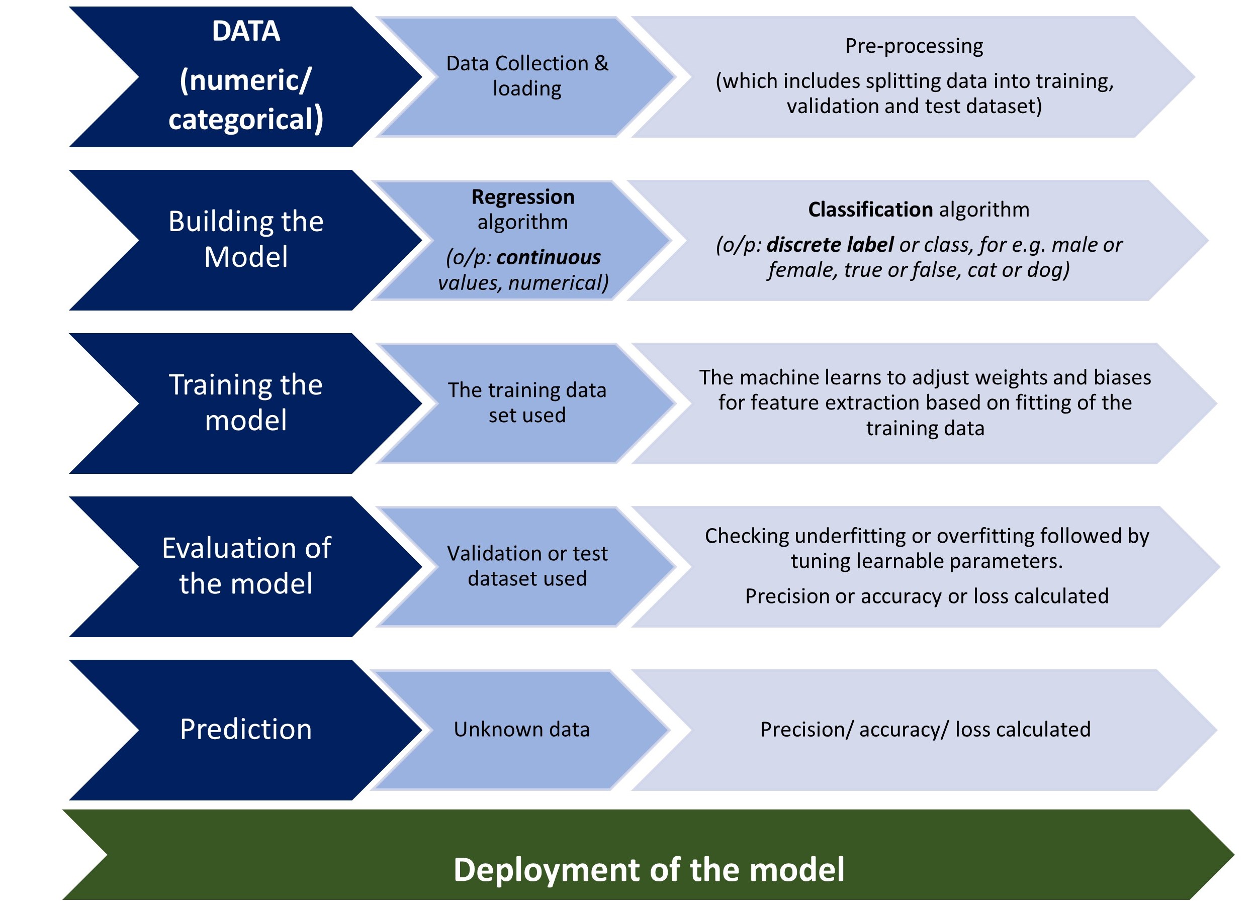 Schematic Diagram of a basic ML framework
I will now walk you through the process of building a deep learning model for image classification.
❶Assigning labels (phase) to the collected microstructures
The given dataset contains four types of microstructures:
❷ Identifying the microstructure and splitting the dataset into training and test data (~80:20)
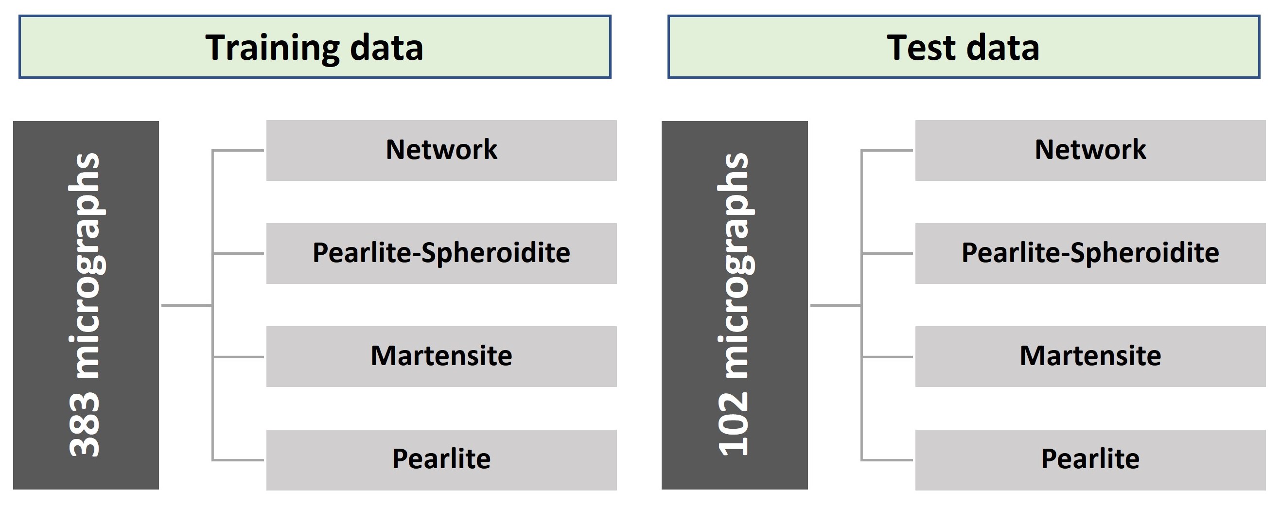
First, the four types of microstructures of steel, namely network, pearlite-spheroidite, martensite and pearlite, are manually identified from the image dataset. Further, they are grouped and stored in four folders and split into training and test data. A folder structure diagram is shown below for clarity.
❸ Loading the image dataset in Python
Begin with importing the relevant Python libraries.
import tensorflow as tf
from tensorflow import keras
from keras.preprocessing.image import ImageDataGenerator
We now need to load the above four folders containing images in Python. For that, I used Keras , written in Python and used mostly in neural networks.
To load the folders, apply keras.preprocessing.image.ImageDataGenerator class.
Training set
train_datagen = ImageDataGenerator(rescale = 1./255)

train_set = train_datagen.flow_from_directory('/Users/saswa/Documents/Joyita_2023/MDXp_content/Tutorail4_UHCSD/UHCSD_ML/Data_steel/Train_set/',
                                               class_mode='categorical',
                                               classes = ['Network','Pearlite_Spheroidite','Martensite', 'Pearlite'],
                                                 target_size = (64, 64),
                                                 batch_size = 32,
                                                 color_mode ='grayscale')
train_set.class_indices
Did you notice the option 'rescale' in ImageDataGenerator? 'Rescale' helps in the normalization of image pixels ranging from 0-255 to 0-1 to ease the processing of models.
Output
Found 383 images belonging to 4 classes.

{'Network': 0, 'Pearlite_Spheroidite': 1, 'Martensite': 2, 'Pearlite': 3}
Test set
test_datagen = ImageDataGenerator(rescale = 1./255)
test_set = test_datagen.flow_from_directory('/Users/saswa/Documents/Joyita_2023/MDXp_content/Tutorail4_UHCSD/UHCSD_ML/Data_steel/Test_set/',class_mode='categorical',
                                            classes = ['Network','Pearlite_Spheroidite','Martensite', 'Pearlite'],
                                            target_size = (64, 64),
                                            batch_size = 32, color_mode ='grayscale')
Output
Found 102 images belonging to 4 classes.
❹ Building Convolutional Neural Network (CNN)
Aim of the model is to identify or, more appropriately in ML language, 'classify' the micrographs.
CNN is a deep learning algorithm used for images, and it consists of multiple layers arranged sequentially.
Code
cnn = tf.keras.models.Sequential()A graphical representation of a typical CNN architecture will help you understand the coding steps for building the same.
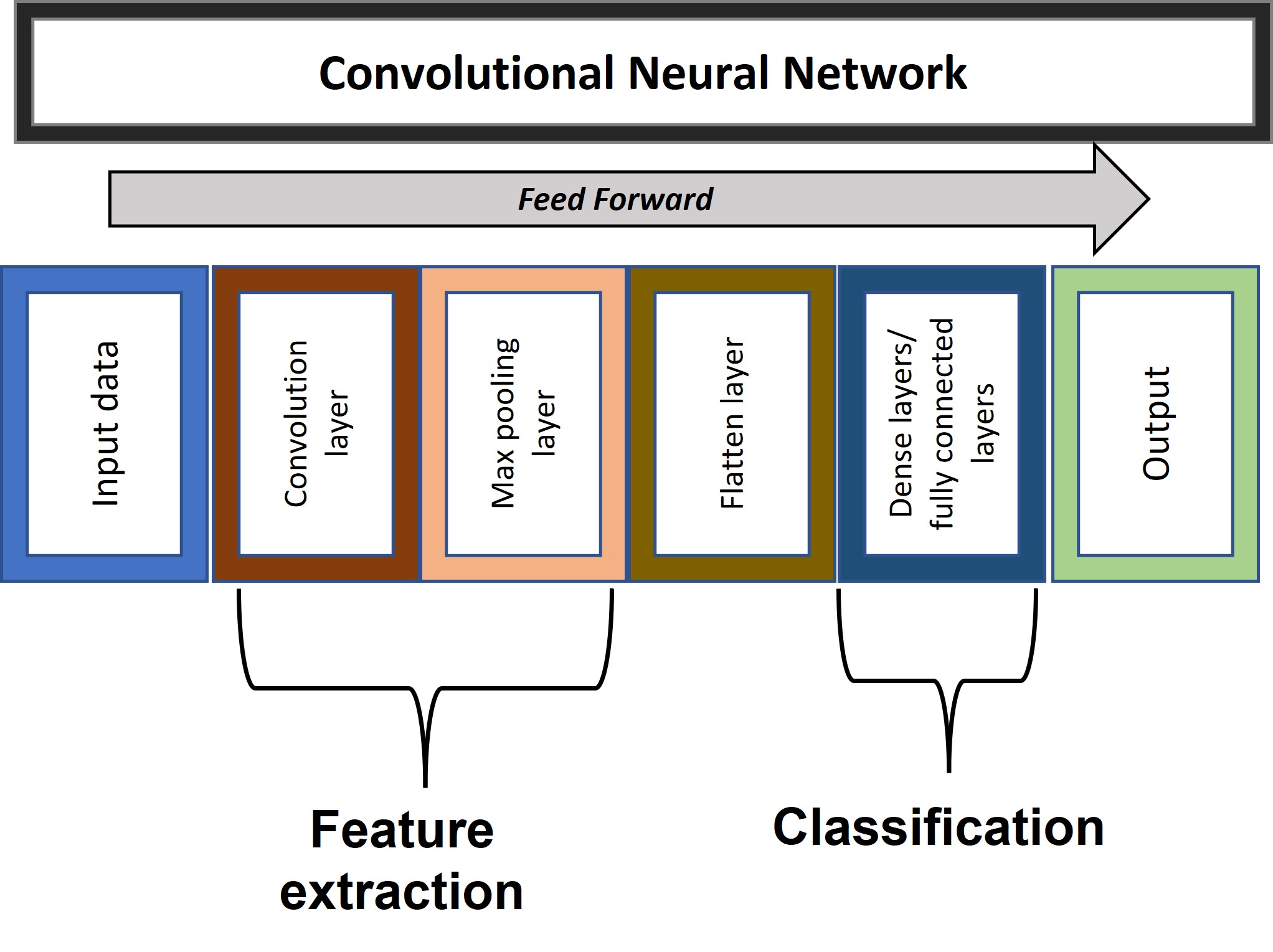
Layer 1: 2D Convolution layer
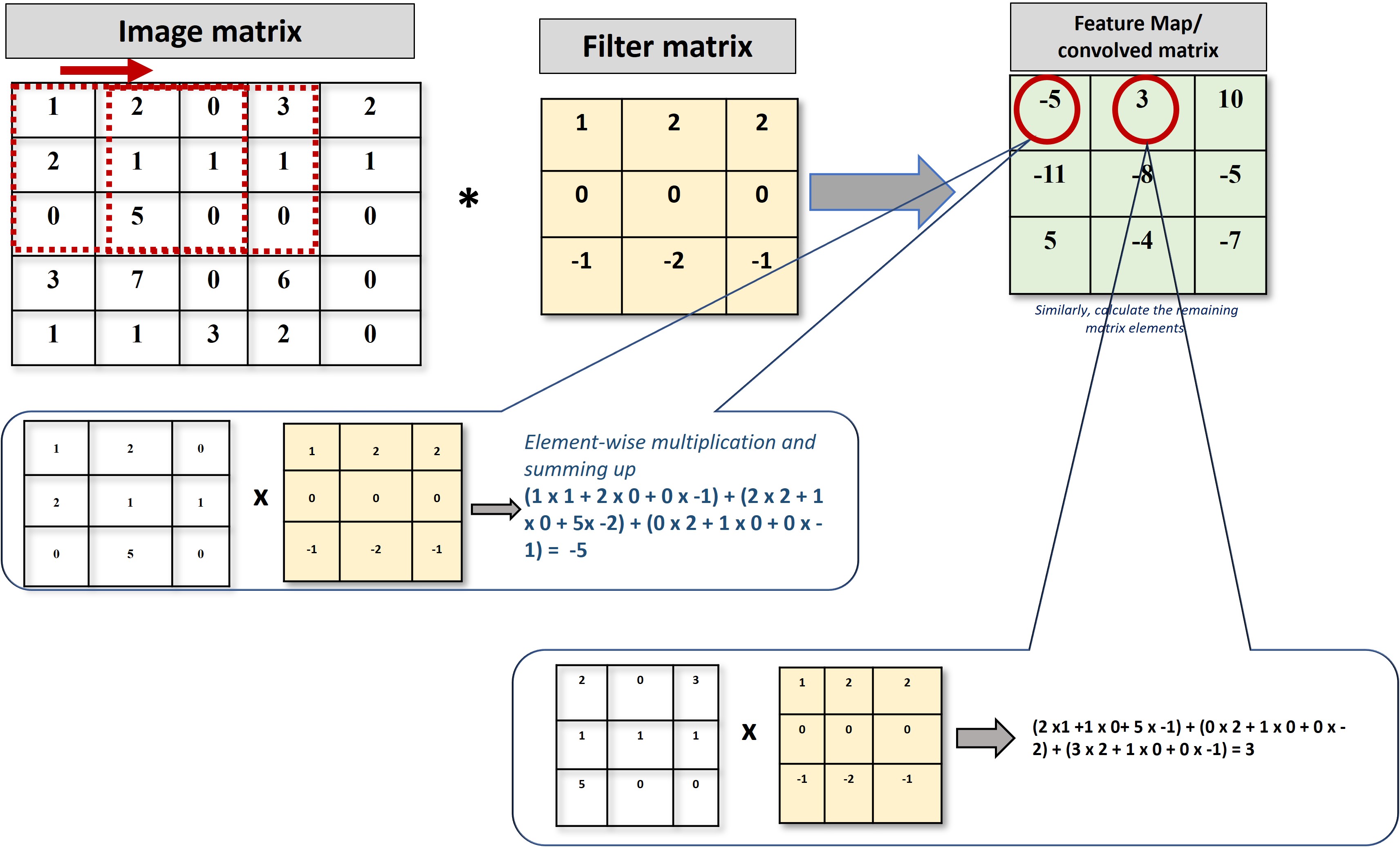
Let us begin with a convolution operation on the image matrix (64 x 64) with 3 x 3 filter and reLU (rectified linear unit) activation function. The convolution of the image matrix with the filter matrix will generate a convolved matrix also known as feature map or activation map . As the name suggests, a feature map reveals the characteristic features of an image which can be used to demarcate or 'classify' different images.
I am sharing a schematic diagram of the convolution operation on an image matrix and a filter matrix for understanding the math followed by the code.
Code
cnn.add(tf.keras.layers.Conv2D(filters = 64, kernel_size =3, activation = 'relu', input_shape = [64, 64,1]))Layer 2: Max Pooling layer
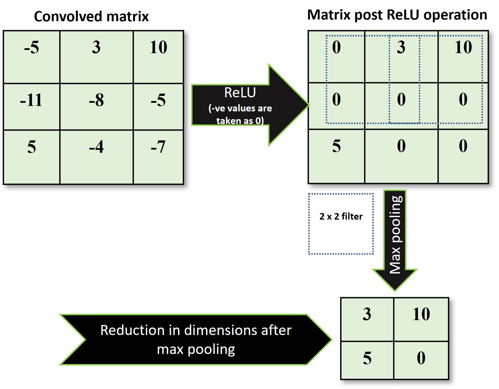
The Convolution layer is followed by a max pooling layer, where the maximum value of the feature map region coinciding with the kernel/ filter is considered. A graphical representation will help to visualize this statement more clearly. As we can see, this operation further downsizes the input matrix.
Code
cnn.add(tf.keras.layers.MaxPool2D(pool_size = 2, strides =2))Layer 3 & 4
In a similar way, I introduced the second convolution layer followed by a max pool layer.
Code
cnn.add(tf.keras.layers.Conv2D(filters=64, kernel_size=3, activation='relu'))
cnn.add(tf.keras.layers.MaxPool2D(pool_size=2, strides=2))
Layer 5: Flatten layer
Inserting this layer converts the max pooled feature maps into a single linear vector.
cnn.add(tf.keras.layers.Flatten())Layer 6 & 7: Dense layers
Dense layers are required to classify images. The input of the flattened layer is fed into the dense layers to give the final output.
I have arranged two dense or the fully connected layers. The final layer has four output neurons for four classes with softmax activation function which will give the output probability.
cnn.add(tf.keras.layers.Dense(units = 128, activation ='relu'))
cnn.add(tf.keras.layers.Dense(units=4, activation='softmax'))
Set the optimization algorithm and loss function
There are several optimization algorithms in machine learning and deep learning determining the model performance. I have employed the ADAptive Moment estimation algorithm (ADAM) for optimization of the current CNN and the loss function is calculated using cross-entropy loss function.
The loss function is based on the softmax activation function, which converts the input vector into a probability distribution. The cross-entropy function evaluates these probabilities by comparing them with their ground truths.
loss_fn = tf.keras.losses.CategoricalCrossentropy(from_logits=True)
optimizer = tf.keras.optimizers.Adam()
Model Summary
To view the summary of the constructed CNN model, use summary method of the model class of Keras.
cnn.summary()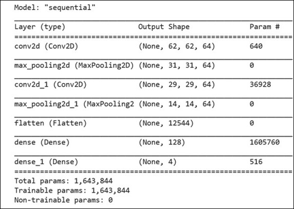
We can get the following information from the model summary table:
The calculations for the trainable parameters and output shape of each layer are elucidated in this link.
❺ Fitting and training CNN with training data
The model is finally trained using the training dataset and validated with test data to check for the accuracy of the model and calculate the loss accordingly.
Here is the coding for the same:
cnn.fit(x = train_set, validation_data = test_set, epochs = 50)Epoch 1/50
12/12 [==============================] - 3s 203ms/step - loss: 1.3413 - accuracy: 0.3922 - val_loss: 1.2195 - val_accuracy: 0.4216
Epoch 2/50
12/12 [==============================] - 1s 107ms/step - loss: 1.1126 - accuracy: 0.5332 - val_loss: 1.1015 - val_accuracy: 0.5196
Epoch 3/50
12/12 [==============================] - 1s 108ms/step - loss: 0.9976 - accuracy: 0.5755 - val_loss: 1.1248 - val_accuracy: 0.4608
Epoch 4/50
12/12 [==============================] - 1s 109ms/step - loss: 0.9533 - accuracy: 0.6044 - val_loss: 1.1439 - val_accuracy: 0.5196
Epoch 5/50
12/12 [==============================] - 1s 106ms/step - loss: 0.9095 - accuracy: 0.6343 - val_loss: 1.0869 - val_accuracy: 0.5000
Epoch 6/50
12/12 [==============================] - 1s 110ms/step - loss: 0.8433 - accuracy: 0.6880 - val_loss: 0.9997 - val_accuracy: 0.5392Understanding important coding terms
You will notice that I used 50 epochs during training the model. The question which immediately pops into our mind is what is an epoch?
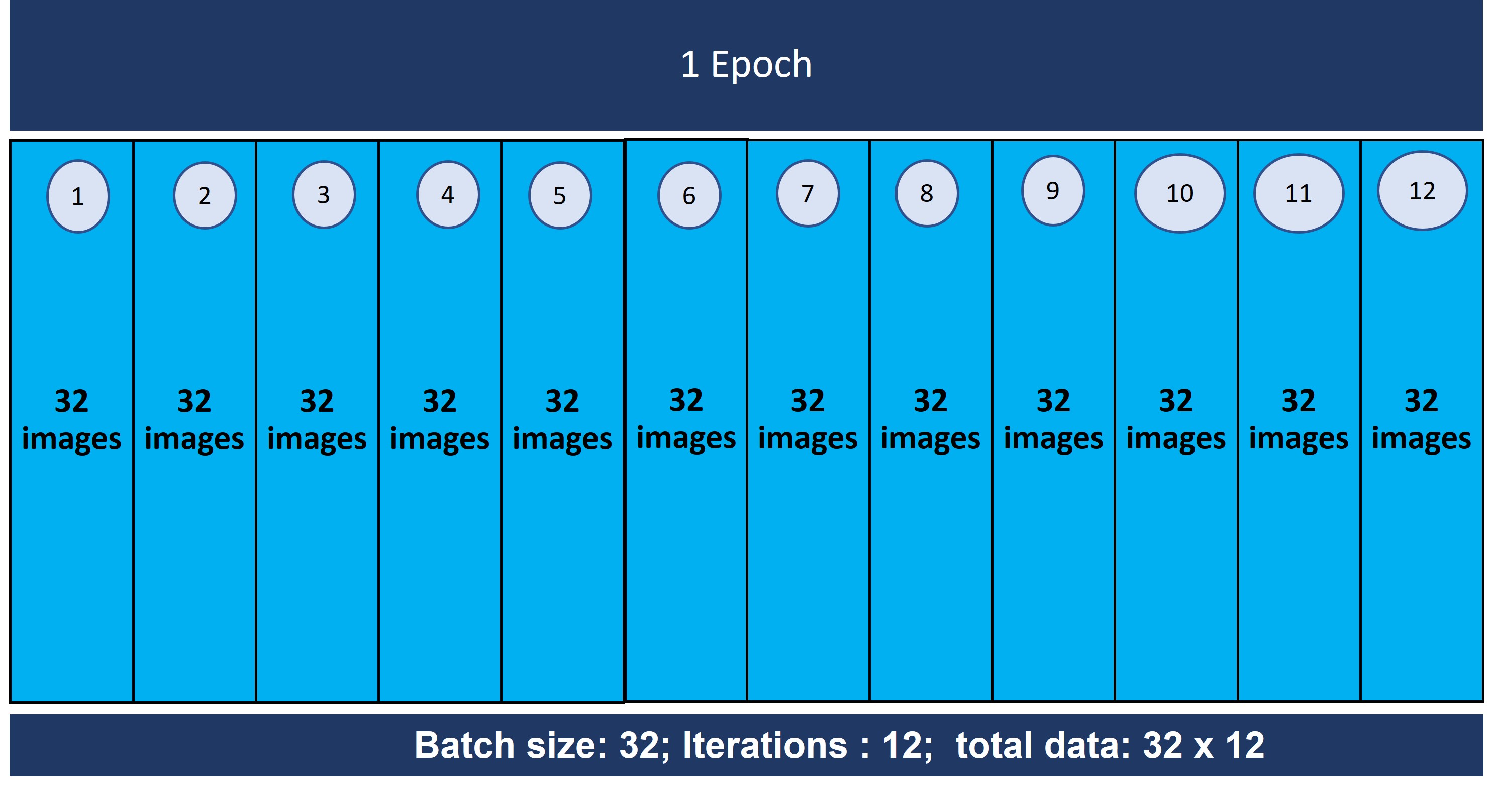
In simple words, an epoch is dataset iterations. In one epoch, the entire dataset is passed forward and backward through the neural network for updating weights and biases required for minimization of error and thereby enhancing the accuracy of the predictive model.
In this particular case, we observe that the whole training dataset is being run 12 times (iterations) in each epoch. Let me explain why the model has taken 12 repetitions.
We have seen that the training dataset consists of 383 images or data points. I assigned a value of 32 to the 'batch_size' while loading the dataset. This means only 32 out of 383 data will be passed at a time through the neural network. In this way, the whole dataset set is divided into 12 batches (383 ÷ 32). This calculation justifies 12 iterations in one epoch in the discussed model.
Below is the schematic diagram portraying the concept of an epoch, batch size, and iteration for understanding.
Validation data is used to evaluate the loss at the end of each epoch.
❻ Making Predictions
Finally, we use the predict method to make prediction for an unknown data. Let’s try to predict an untrained network microstructure using the above trained CNN model.
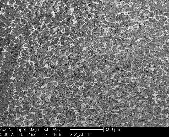 Untrained network microstructure
The snapshot of coding for loading an unknown image data and predicting its class is displayed below:
import numpy as np
from keras.preprocessing import image
from keras_preprocessing.image import load_img
from keras_preprocessing.image import img_to_array
#from tensorflow.keras.utils import load_img
#from tensorflow.keras.utils import img_to_array
test_image = load_img('/Users/saswa/Documents/Joyita_2023/MDXp_content/Tutorail4_UHCSD/UHCSD_ML/Data_steel/single_prediction/net.tif', target_size = (64, 64),color_mode = 'grayscale')
test_image = img_to_array(test_image)
test_image = np.expand_dims(test_image, axis = 0)
result = (cnn.predict(test_image) > 0.3).astype('int')
print(result)
train_set.class_indices

# >0.3 is the decision threshold of predictions
Output
[[1 0 0 0]]

{'Network': 0, 'Pearlite_Spheroidite': 1, 'Martensite': 2, 'Pearlite': 3}
Explaining the prediction output
The entire image dataset is divided into four classes stored as a python dictionary with key-value pair.
{'Network': 0, 'Pearlite_Spheroidite': 1, 'Martensite': 2, 'Pearlite': 3}
The prediction output is [[1 0 0 0]].I converted the prediction probability into a crisp binary prediction by applying astype(int) method of pandas where 1 and 0 represents true and false repectively. So you can read the result as [true false false false].
The first class in the dictionary is 'Network' and the prediction of 1 indicates correct output unlike the other three classes where the prediction output is 0 indicating their absence or non-occurrence. Thus, the model could correctly classify the unknown microstructure as network.
Wrapping up
Click here to avail the entire code and references for the used dataset.
Links to get the training and test images:
Note that I used Jupyter Notebook to run this code. The same code can be run in Google Colab. However, in the latter environment, loading image folders requires a few more lines of code. Please take a look at my tutorial on the same.