Materials Data Mining via Image Processing of Micrographs - I
by Joyita Bhattacharya
Background
In my post 'Uncovering the Potential of Materials Data using Matminer and Pymatgen', I discussed the concept of materials tetrahedron-the basic framework for developing materials for various technological usage. The vital parameters occupying the vertices of the tetrahedron are process, structure, property, and performance.
Structures are characterized based on a characteristic length scale that can vary from a few angstroms (1 Angstrom = 10-10 m) to hundreds of micrometers (1 micrometer = 10-6 m). The length scales are used to discern features under a microscope. With very powerful high-resolution microscopes such as this one, one can identify features as small as atoms or even smaller.
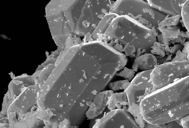
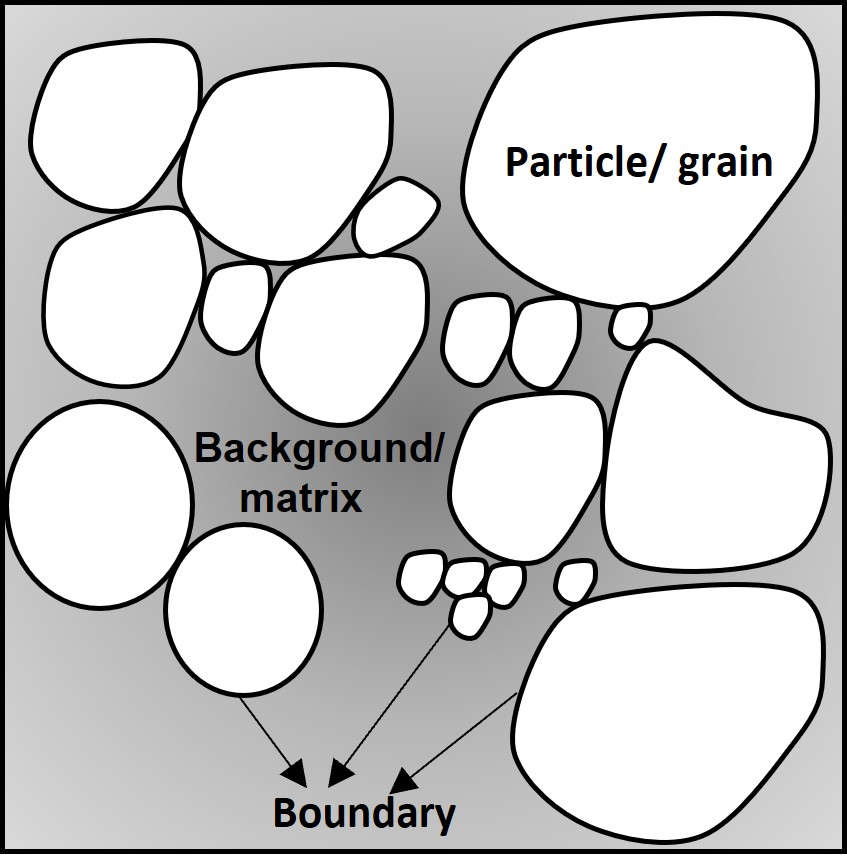
Micron and submicron-sized features, known as microstructures, are captured as images or micrographs using different types of microscopes. These microstructures store a wealth of information essential to the understanding of properties and performance of materials. We can use machine learning/deep learning to mine important features from these images. A typical microstructure contains features that are distinguishable based on pixel intensity or contrast. Some of the important features are boundaries or interfaces that separate different domains (also termed as particles or grains). These domains can vary in shape, size, orientation, size distribution and spatial arrangement (collectively termed as morphology). These features affect the properties of materials.
Even though these features can be studied using other materials characterization techniques, the advantage of microscopy is visualization. Since 'seeing is believing', micrographs provide more credible explanation for the behavior of materials. Processing of micrographs reveal qualitative and quantitative features. Say, for example, if we want to go for quantitative particle size and morphology measurement, precise identification of edges becomes necessary. Moreover, edge detection also helps in investigating the interface structure between particles. In some materials (especially alloys), some elements might segregate at interfaces affecting properties such as strength, conductivity.
Edge detection by manual observation is a tedious task and involves various human errors. To minimize such errors, one needs to automate such a process. Automation of the process requires implementation of robust digital image processing and data mining algorithms. Now that I have highlighted the importance of digital image analysis of micrographs, let me walk you through some of the basic processing steps. I have used the open-source python-based library, scikit-image for demonstration. You can also explore OpenCV, PIL for the same purpose.
Viewing the image and obtaining shape
The code snippet below shows how to read an image and find its dimensions or 'shape'. The shape attribute yields the dimensions of the image in the form of a tuple. In this current micrograph, it is (1800, 1500)-the height and width being 1800 and 1500 pixels, respectively. Note that it is a grayscale image since the third item in the tuple is not mentioned and takes the default value of 1.
 p = io.imread("Particles.jpg")
 p.shape
General processing steps: Denoising, Sharpening and brightness adjustment of image

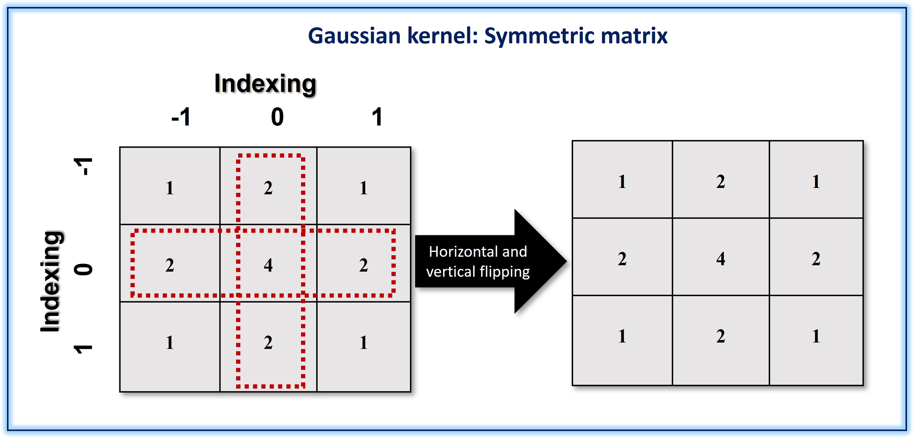
Refinement of an image matrix for denoising, sharpening, edge detection mostly involves convolution operation with a filter/kernel matrix. The convolution operation involves first flipping of the 2D filter (kernel) horizontally and vertically followed by element-wise multiplication and addition of the image matrix . Note that in case of symmetric kernel matrix, flipping is not necessary.
Here, I am going to consider two filters-Gaussian and Median for showing the noise reduction in images associated with and without convolution respectively.
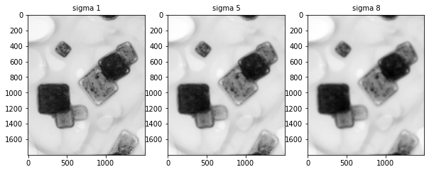
The linear Gaussian filter operates on the image matrix by convolution. The attribute 'sigma' is the standard deviation in the Gaussian filter. A higher value of sigma leads to more blurriness.
Median filtering is a nonlinear process. When a filter window slides along the image matrix, the median pixel value of the said matrix is taken as the output signal. A graphical representation is shown for better understanding.
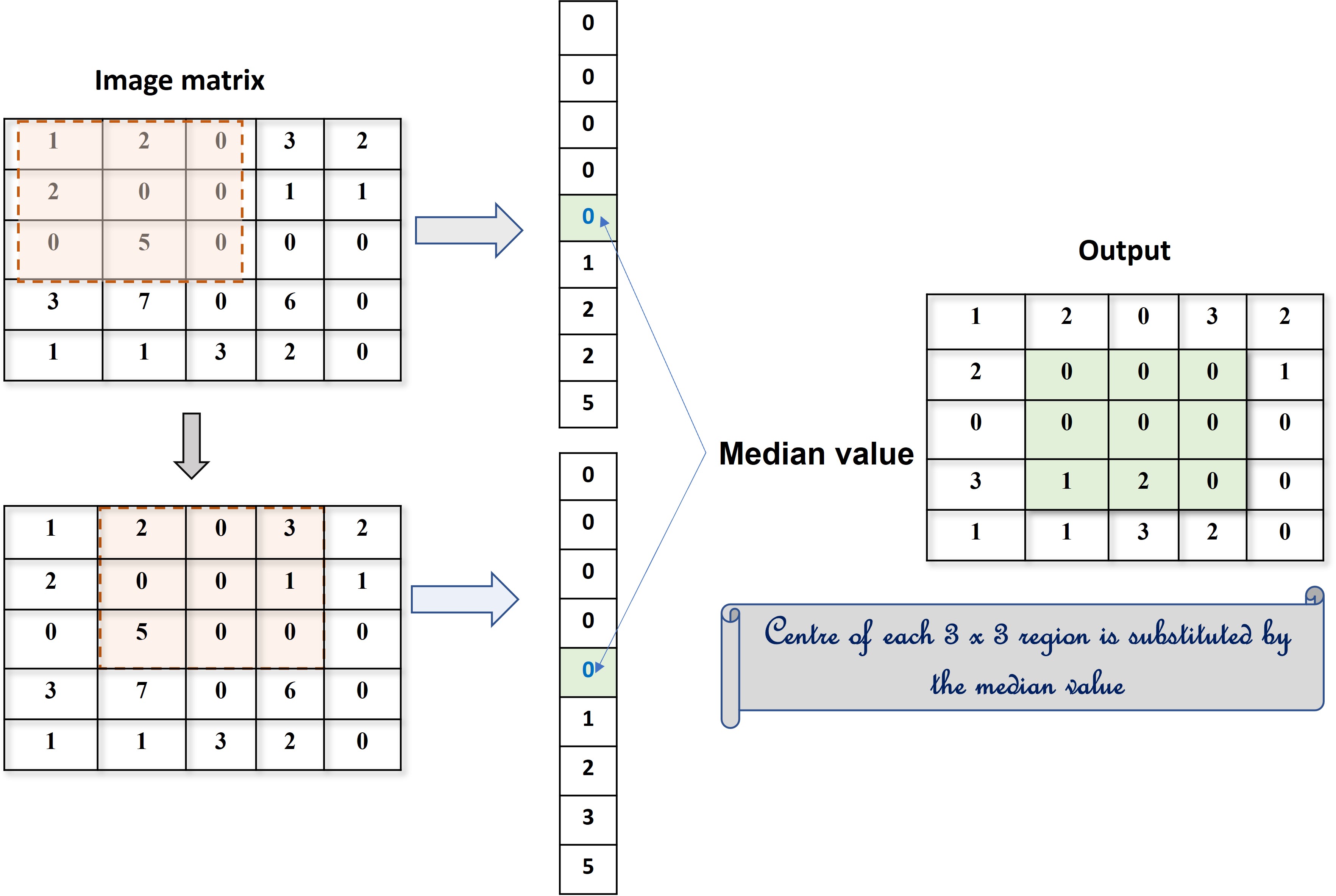
This filter is preferred over the Gaussian filter while removing electronic noises such as salt and pepper type. While Gaussian smoothing causes blurring of edges, median smoothing preserves them.
In contrast to denoising, we can sharpen a defocussed or blurred image to identify the features in it accurately using the 'unsharp_mask' function of the 'filters module' of skimage. The code snippet along with input (defocussed image) and output (sharpened) images are displayed below for comparison.
Sharpimg = filters.unsharp_mask(p, radius = 20.0, amount = 1.0)
fig, ax = plt.subplots(nrows =1, ncols =2, sharex = True, figsize =(15,15))
ax[0].imshow(p, cmap = 'gray')
ax[0].set_title("Original", fontsize = 10)
ax[1].imshow(Sharpimg, cmap ='gray')
ax[1].set_title("Sharpened",fontsize = 10)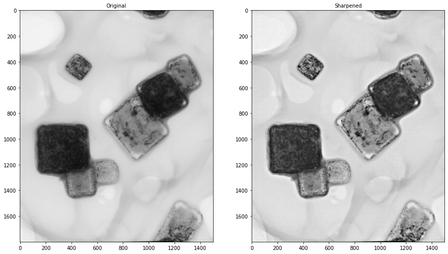
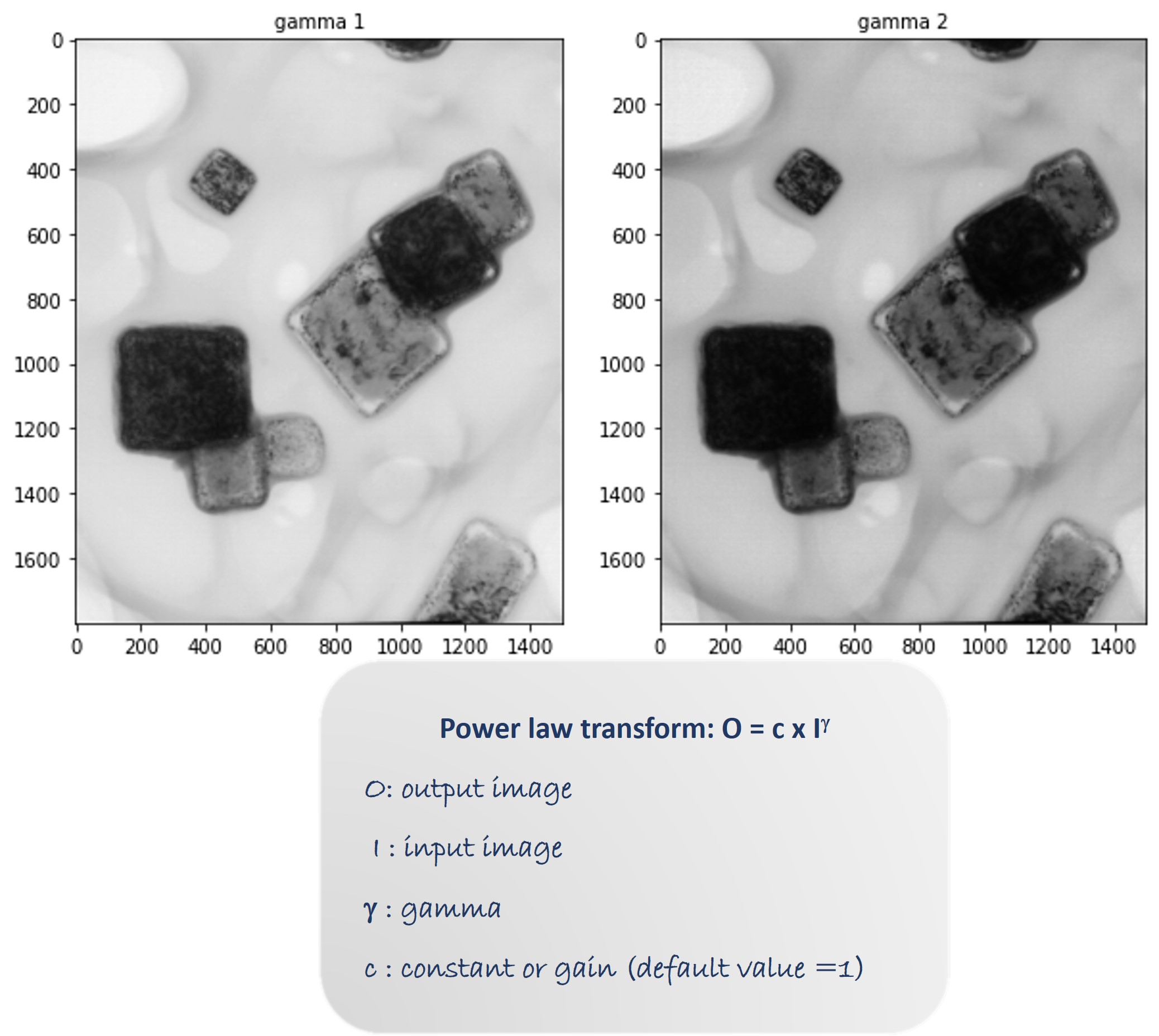
Sometimes, adjusting the brightness also brings out the clarity in an image for feature detection and this can be done using the function 'adjust_gamma' of the 'exposure module' of skimage. The gamma-corrected output image is obtained by applying the power-law transform.
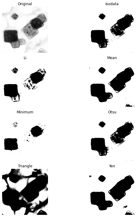
Thresholding for image segmentation: Creating Binary image
Thresholding is required when we need to separate the image background from the foreground based on pixel intensity. For example, in the case of superalloy (material for jet engines of airplanes, gas turbines) microstructures, the background is the base metal, and the foreground is comprised of precipitates which imparts super strength to this type of material. Sometimes, the background can be just the sample holder used to load the sample for investigation under microscopes. The image used for thresholding, in this case, shows four-corned particles on a transmission electron microscope (TEM) grid/ holder. Different types of thresholding methods are applied to distinguish the background (TEM grid) from the particles. For the given micrograph, we find the mean thresholding is doing a better job than the other methods by clearly forming a binary image as shown in the code output snippet.
The above methods are some of the preliminary steps to obtain a noise-free image before subjecting it to further processing for extraction of meaningful features both qualitative and quantitative. As mentioned at the beginning of this post, particle size is one of the vital parameters/ features controlling the properties of a material. To estimate the particle size from an image, we need to detect the edges of the particles vividly. And this task becomes easy using various edge-detection filters. Here, I will be discussing a few of them.
Edge Detection using Roberts, Sobel, Canny filters
Roberts and Sobel filters are 2 x 2 and 3 x 3 convolution kernels respectively. Both filters have x and y components for horizontal and vertical edge detection. Code snippets for the Sobel kernel operations along with the corresponding outputs are displayed below.
from skimage.filters import sobel,sobel_v, sobel_h
p_sobel = sobel(p_g, mode='reflect')
p_sobel_v=sobel_v(p_g)
p_sobel_h=sobel_h(p_g)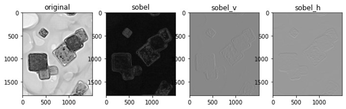
Canny filter does a multi-tasking job by smoothing, gradient approximation by Sobel operators, detecting the edges using hysteresis thresholding. The function 'canny' has parameters such as sigma for the Gaussian smoothing and low and high threshold.
Gabor Filter for detecting Edge orientations
This linear filter captures the texture or orientation distribution of features in the microstructure. Orientation distribution determines the uniformity of materials property. Random orientation of particles/grains leads to uniform/ isotropic properties while orientation in a particular direction, technically termed as preferred orientation, gives rise to anisotropic properties. The complex sinusoid component of the Gabor filter provides information related to orientation. The output of the said filter has both real and imaginary components. To know more about Gabor filters, please click here.
Let's try to generate a bank of Gabor filters with 0°, 60°, 90°, and 120° orientations and apply them to an original transmission electron micrograph showing particles at different orientations . I am sharing the code snippet along with the output filtered images below. We can clearly see the orientations (highlighted in yellow dotted line coinciding with particle edges) in the respective filtered images. Please note that the real components of the filtered images are displayed.
p_gabor =[]for degree in (0, 60, 90, 120):
    real,imag = filters.gabor(p, frequency=0.05, theta =(degree* (np.pi)/180))
p_gabor.append(real)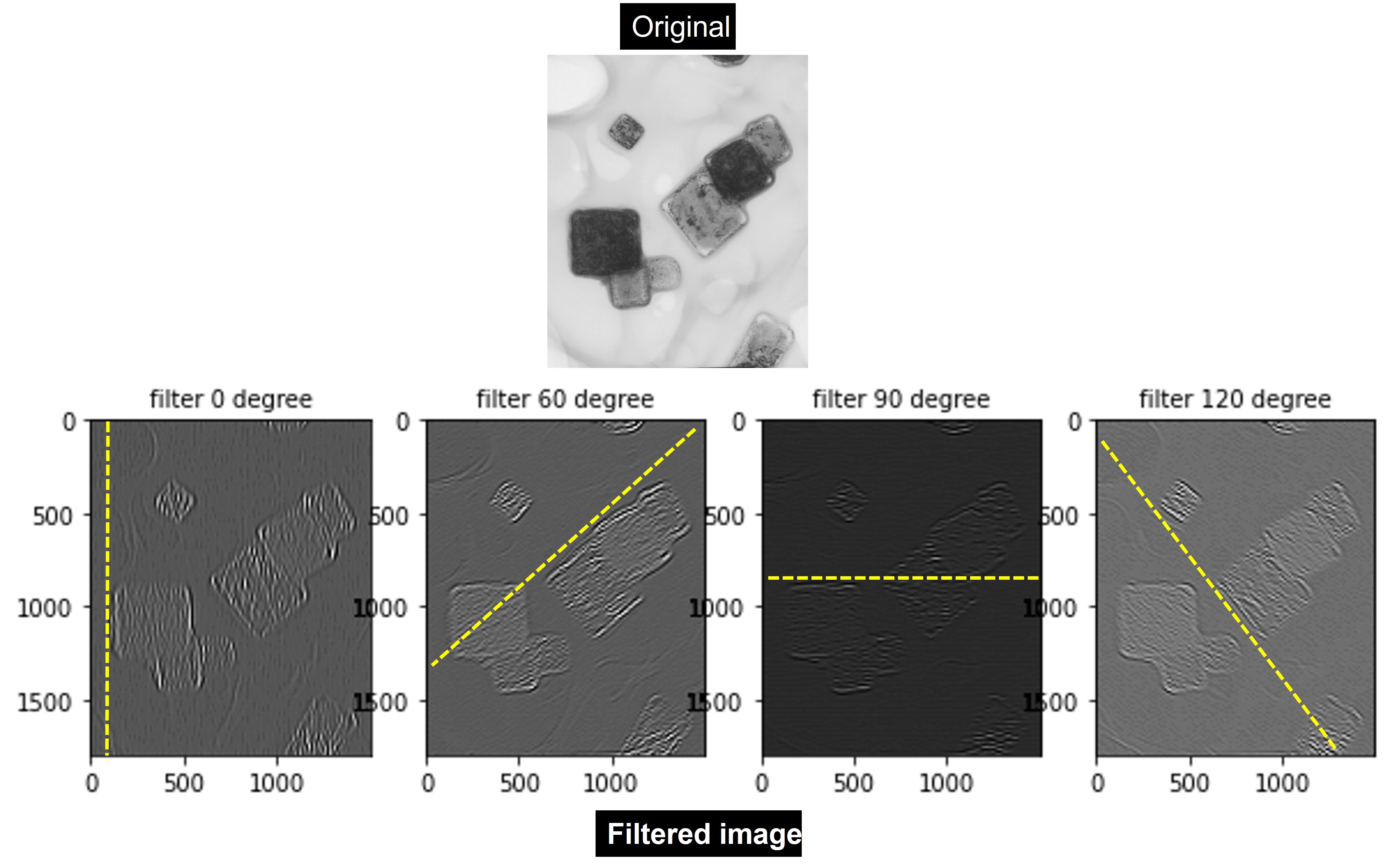
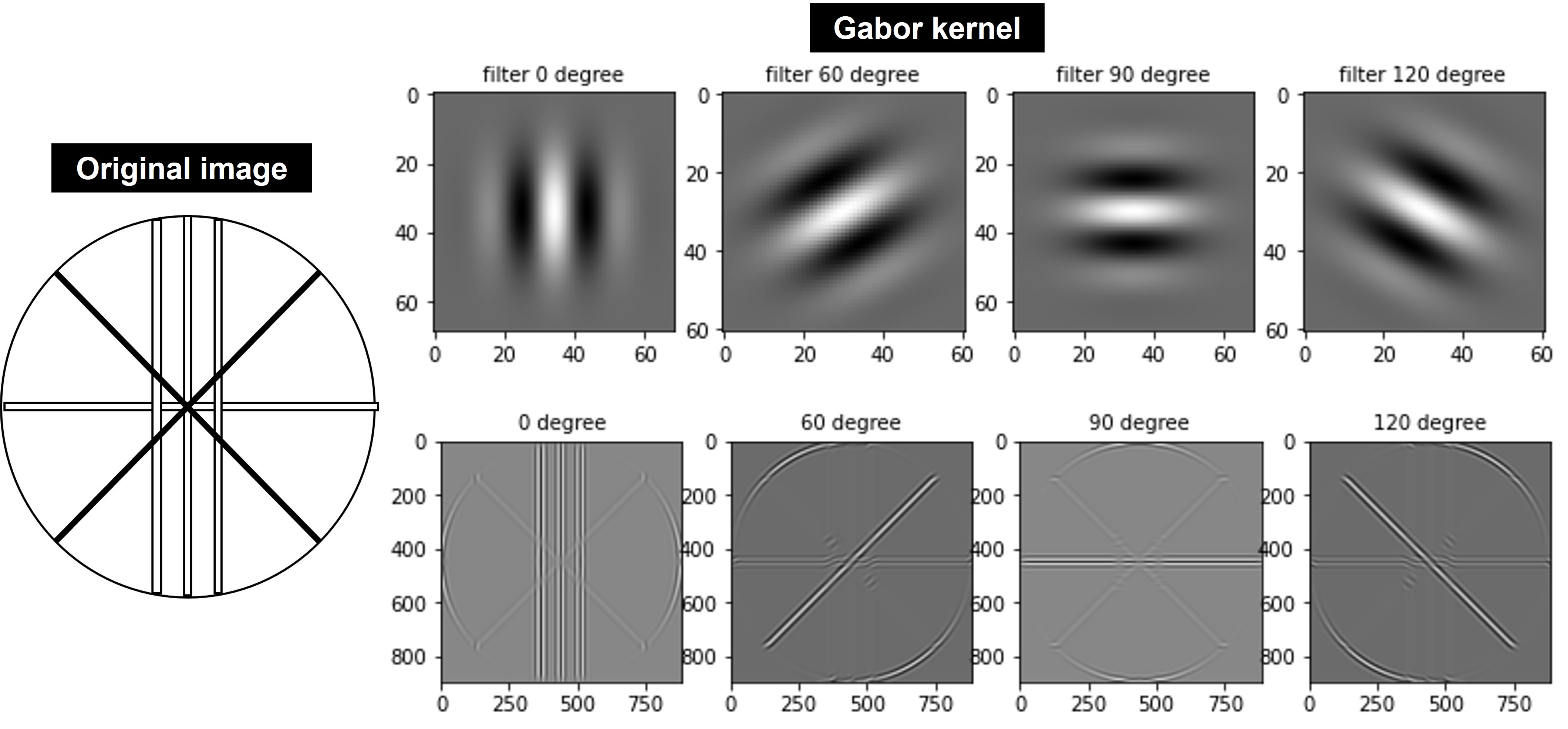
We can also apply the Gabor kernel for extracting information on orientations. A bunch of Gabor kernels of different orientations is generated and then they are allowed to interact with the image matrix to resolve the edges in the corresponding directions, as shown in the below snapshot.
Click here to get the entire code for the basic image processing from my GitHub repository.
Summary
Mining qualitative and quantitative features is the key to understanding the microstructure-informed properties of materials. Besides, data from biological imaging is the backbone to healthcare industry. Hence, judicious processing of these micrographs is crucial.
Despite the availability of several commercial image processing software, generating your own algorithms for the same purpose is cost-effective plus flexible. And, most importantly, opens the gate for automation via machine learning.
In this post, I have explained some basic processing steps for extracting information qualitatively, such as detecting particle edges and orientations. However, complete data extraction from micrographs also entails a quantitative assessment of relevant features, which I will be discussing in my next post.
Until then, happy image processing!!