Materials Data Mining via Image Processing of Micrographs -II
by Joyita Bhattacharya

Background
My previous post 'Materials Data Mining via Image Processing of Micrographs-I' explained some of the basic and crucial steps of micrograph processing for the identification of features. As stated earlier, micrographs capture fine micron/sub-micron sized features of materials that can significantly impact their properties. Here, I will be discussing the quantitative assessment of one such feature-'particle size' using scikit-image.
Measurement of parameters
Case Study 1: Retrieving individual particle size from clusters applying Watershed algorithm
Let me start by showing a synthetic micrograph with overlapping particles of different shapes and sizes. We first separate individual particles from clusters/ agglomerates. Then we measure the size of these separated particles. De-agglomeration of particles is achieved with the aid of a watershed algorithm-a type of image segmentation method. I am sharing a step-by-step guide for the said activity.
Step 1: Importing necessary libraries and loading image
# IMPORTING LIBRARIES
import numpy as np
import pandas as pd
import matplotlib.pyplot as plt
from scipy import ndimage as ndi
from skimage import io, color
from skimage.segmentation import watershed
from skimage.feature import peak_local_max

# LOADING IMAGE
im1 = io.imread("O3.jpg")
plt.imshow(im1, cmap ='gray')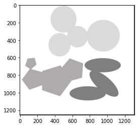
The image has several clusters of particles, and its dimension is represented by a tuple (1254, 1313, 3). While the first two elements of the tuple indicate height and width, the third one tells us the number of channels (number of colors). This image is an RGB image having three channels/colors.
Step 2: Converting to grayscale image
I have applied the function rgb2gray imported from the color module of skimage to convert the RGB image to grayscale.
Step 3: Thresholding to get a binary image
The mean thresholding method is found to be most suitable for this image after it is subjected to other thresholding methods using the try_all_threshold function.
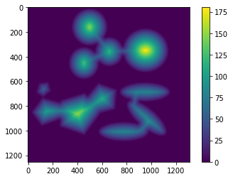
Step 4: Computing the Euclidean distance transform
The Euclidean distance is a measure of the closest distance between any two pixels in the image. Each pixel of the image is categorized as either a source/background pixel (with zero intensity) or an object pixel (with non-zero intensity). We observe a descending gradient in Euclidean distances from the center of any object to the background. This is beautifully captured in the distance map obtained from the image:
Step 5: Finding local peaks and watershed line
A watershed, geographically speaking, is a highland that separates drainage basins. We apply the same concept to image segmentation for clusters of particles/objects. In this case, the pixel intensities of the boundaries of an individual object in the cluster constitute the watershed divide, separating them from one another.
We first locate the coordinates of the peaks (local maxima) of the particles by applying the function peak_local_max. We use the output of this function as markers in the watershed function. We label these markers for each particle in the image. These markers constitute the watershed line that separates individual particles from an agglomeration. The code snippet for the task is shown below.
coords = peak_local_max(distance, min_distance =100)
mask = np.zeros(distance.shape, dtype=bool)
mask[tuple(coords.T)] = True
markers,_= ndi.label(mask)
Step 6: Image segmentation applying watershed algorithm
Finally, applying the watershed algorithm with parameters such as inverse distance transform image, markers, and mask (binary image), we obtain separate particles. The individuality of these particles in clusters is displayed in different colors by applying the matplotlib colormap.
individual_particles = watershed(-distance, markers, mask=binary)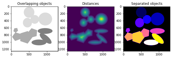
Case Study 2: Measurement of properties-Particle Size and Particle size distribution
Let us continue with the above image where we applied the watershed algorithm to separate particles from clusters. We now proceed with the measurement of particle size.
Role of scale factor in an image
Before going through the details of the computation of values of features/ parameters, we need to understand the concept of 'scale' in an image. Scale factor in any image gives an idea of the measure of the objects/features. A digital image is comprised of tiny dots called pixels. The size of the pixel defines the resolution of the instrument used to take the pictures.
A scale-line or bar of a few pixels representing a certain value in terms of kilometers/centimeters/millimeters/micrometers/nanometers is provided on any image depending on the sizes of actual physical objects captured in the image. For instance, a Google map has a scale bar either in miles or kilometers. Conversely, micrographs have scale bars in micrometers/ nanometers as they capture small length-scale features of materials.
It is impossible to measure the features of an image without a scale bar. Thus, an image with quantifiable features should always contain a scale bar.
Size measurement using regionprops function of skimage.measure module
The code for measurement applying regionprops function to the labeled image regions is presented below.
from skimage.measure import label, regionprops, regionprops_table
label_img = label(individual_particles, connectivity = im2.ndim)
props=regionprops(label_img, im2)
for p in props:
display('label: {} area: {}'.format(p.label, p.area))
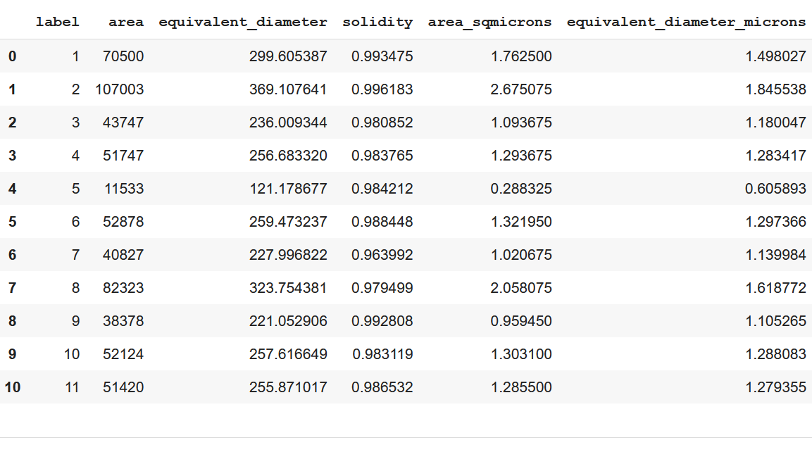
props_t = regionprops_table(label_img, im2, properties='label','area', 'equivalent_diameter','solidity'])
df = pd.DataFrame(props_t)The properties, such as area, equivalent diameter, and solidity, are tabulated as a pandas-compatible table using the regionprops_table function. A scale of 0.005 microns per pixel is considered to calculate the size of particles.
The parameter 'particle size distribution' becomes significant when there are particles of varied sizes in a micrograph. All real-world materials contain innumerable particles (such as polycrystalline metals). Micrographs capture only a small representative region of the material. Particle size, as mentioned at the beginning of this post, dictates several important properties of a material.
Now, the question arises as to whether one should consider the mean particle size or the entire particle size distribution (PSD). Mean particle size is reported for materials having uniformity in particle size, while PSD becomes a vital parameter for materials with particle sizes varying over a range.
The distribution plot of particle size showing D10, D50, and D90 percentile becomes informative and is used as a guidance to understand the behavior of materials. Additionally, it tells us about the uniformity of the parameter by calculating the 'Span' defined as follows.
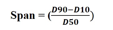
A smaller span value signifies more consistency in particle size. On the other hand, a larger span value implies heterogeneity in the distribution.
I have taken a simulated image below to show the calculation of particle size distribution.
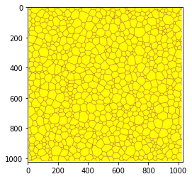
This image shows a considerable number of well-separated individual particles with varying sizes. Since there are no clusters of particles in this image, the step of applying the watershed function is irrelevant. First, we convert this image to grayscale followed by thresholding. We then apply the label function to the binary image to generate a labeled image ( as shown below) displaying particles of different sizes with distinct colors.
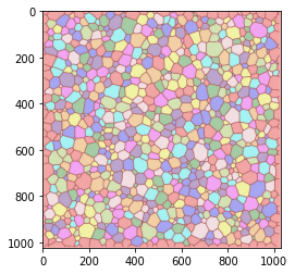
A scale of 4 nanometers per pixel is applied to calculate the equivalent diameter representing the particle size. Note that an equivalent diameter is the diameter of a circle with the same area as the region. We directly compute and tabulate the required properties using regionprops and regionprops_table. The table is then exported as a spreadsheet file. Using the percentile function of Numpy, we obtain the statistical parameters-D10, D50, and D90 percentiles. Accordingly, a span approximately equal to unity is estimated which indicates non-uniformity of particle size for the simulated image. Note that a span closer to zero denotes a more consistent PSD.
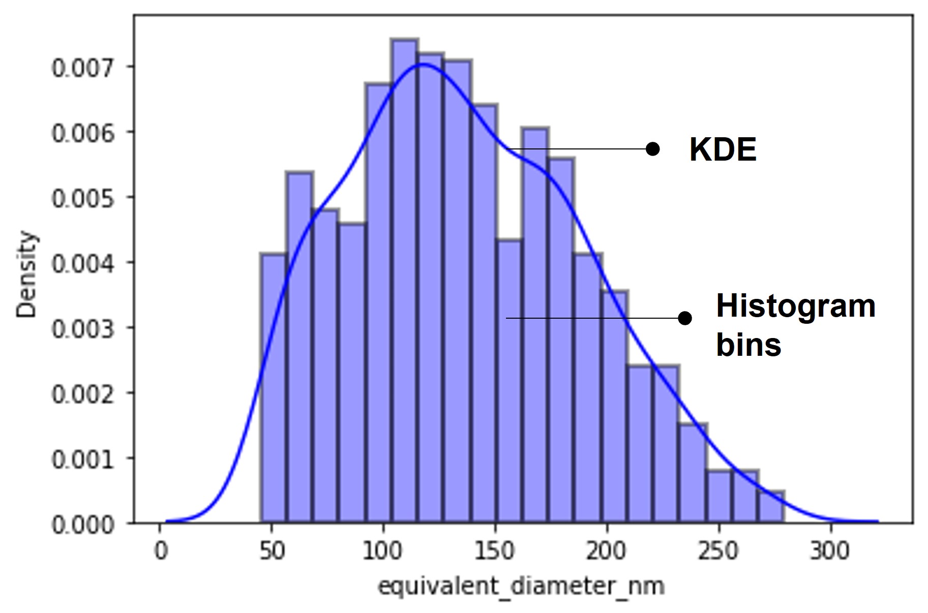
Visualization of particle size distribution
I have used Seaborn-a statistical data visualization library to plot the particle size distribution using distplot function. This function combines the histogram and kernel density estimation (KDE) functions. The figure below shows the particle size distribution plot of the simulated image.
Summary
Quantitative estimation is an essential part of image data processing as it assists in decision-making. Defining a scale bar in an image is mandatory for the quantification of features. Furthermore, an image needs to undergo a set of refinement steps prior to the quantitative analysis.
In this post, I have illustrated the above point by taking two images with the objective of mining particle size data. I demonstrated the necessity of an additional pre-processing step of applying the watershed function to separate the particles for size calculation in the first image with overlapping particles. We would have otherwise landed up with sizes of clusters of particles. This would have been utterly misleading for interpretation of the same vis-à-vis materials property.
The other highlight of this post describes the significance of particle size distribution, rather than a single mean value, for systems (image) containing particles of varied sizes. PSD is an important quantifier for materials with structural heterogeneity (e.g., polycrystalline materials).
I hope this post will help in the calculation of measurable parameters from images that can be incorporated as input for predictive algorithms.
Thanks for reading!