Photo by Jonathan Petersson on Unsplash

Background

SHAP-the acronym for 'SHapley Additive explanations' API can help explore novel materials with desired properties and performance. This concept unveils the contributions of each input parameter to the final output in the machine learning algorithm. Thus the interpretability factor is infused into the machine learning algorithm, which, otherwise, is treated as a black box.

Please refer to my blog to know about SHAP in detail.

In this tutorial, I will walk you through each step of SHAP-aided machine learning for identifying elemental combinations for a potential thermoelectric with an ideal combination of high power factor (PF) and low thermal conductivity (κ or kappa).

Case study: Finding potential thermoelectric compositions with multioutput ML algorithm and SHAP analysis

Data: I have compiled room temperature PF and kappa values of 204 thermoelectric compositions (formulae) in an excel sheet. Click here to see the reference for this dataset.

Step 1: Import and Install relevant Python libraries

A snapshot of the libraries imported is shown below:

import numpy as np
import pandas as pd
from matplotlib import pyplot as plt
from matplotlib.pyplot import figure
from sklearn.ensemble import RandomForestRegressor
from sklearn.model_selection import train_test_split

Install the materials libraries – Matminer and Pymatgen

pip install pymatgen

pip install matminer

Step 2: Loading data

ds_RT = pd.read_csv('Pf_kappa_RT_2.csv')
ds_RT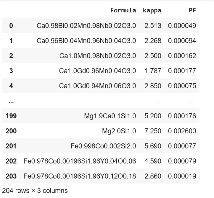

Step 3: Prepossessing data for machine learning

Why preprocessing step is a must activity in this case?

The original data file contains only three variables-Formula, PF and kappa where the latter two are targets/ responses. However, to come up with new composition we need to do a permutation of elements comprising these formulae and incorporate them as input variables/ features. Moreover, we also need the data (amount or elemental fraction) of each element present in a composition.

Therefore, we extract individual element and their elemental fraction from a given formula using the 'Composition' and 'Element fraction' modules of Pymatgen and Matminer respectively.

Here is the snippet of code blocks displaying the breaking down of a formula into its constituent elements and their corresponding element fraction.

Importing Composition and ElementFraction

from pymatgen.core.composition import Composition
from matminer.featurizers.composition import ElementFraction
ef = ElementFraction()
element_fraction_labels = ef.feature_labels()
print(element_fraction_labels)

[H', 'He', 'Li', 'Be', 'B', 'C', 'N', 'O', 'F', 'Ne', 'Na', 'Mg', 'Al', 'Si', 'P', 'S', 'Cl', 'Ar', 'K', 'Ca', 'Sc', 'Ti', 'V', 'Cr', 'Mn', 'Fe', 'Co', 'Ni', 'Cu', 'Zn', 'Ga', 'Ge', 'As', 'Se', 'Br', 'Kr', 'Rb', 'Sr', 'Y', 'Zr', 'Nb', 'Mo', 'Tc', 'Ru', 'Rh', 'Pd', 'Ag', 'Cd', 'In', 'Sn', 'Sb', 'Te', 'I', 'Xe', 'Cs', 'Ba', 'La', 'Ce', 'Pr', 'Nd', 'Pm', 'Sm', 'Eu', 'Gd', 'Tb', 'Dy', 'Ho', 'Er', 'Tm', 'Yb', 'Lu', 'Hf', 'Ta', 'W', 'Re', 'Os', 'Ir', 'Pt', 'Au', 'Hg', 'Tl', 'Pb', 'Bi', 'Po', 'At', 'Rn', 'Fr', 'Ra', 'Ac', 'Th', 'Pa', 'U', 'Np', 'Pu', 'Am', 'Cm', 'Bk', 'Cf', 'Es', 'Fm', 'Md', 'No', 'Lr']

ds_RT['Formula']
Comp = []
for value in ds_RT['Formula']:
  Comp.append(Composition(value))
Comp

[Comp: Ca0.98 Mn0.98 Nb0.02 Bi0.02 O3,
 Comp: Ca0.96 Mn0.96 Nb0.04 Bi0.04 O3,
 Comp: Ca1 Mn0.98 Nb0.02 O3,
 .
 .
 .
 .
 .
 Comp: Fe0.998 Co0.002 Si2,
 Comp: Y0.04 Fe0.978 Co0.00196 Si1.96 O0.06,
 Comp: Y0.12 Fe0.978 Co0.00196 Si1.9]

Addition of "Composition" column to the original dataset

 ds_RT['Composition'] = Comp
 ds_RT

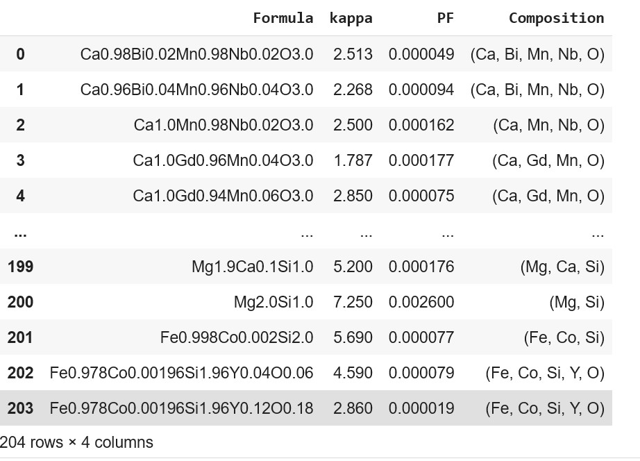
Incorporating individual element and the corresponding element fraction present in a formula using ElementFraction (ef) class of matminer.featurizers.composition module to the dataframe

 ds_RT = ef.featurize_dataframe(ds_RT,'Composition')
 ds_RT

The final refined data, ready for ML, shows a total of 51 columns and 204 rows. Out of 51 variables, 49 are input variables/features and the last two columns representing PF and kappa, are targets.

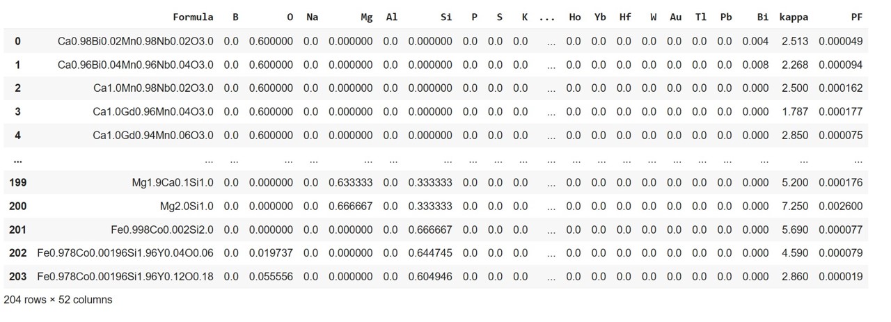
Preprocessing of data is explicitly discussed here.

Step 4: Defining X and y

 X = ds_RT.iloc[:, 1: 50]

 y = ds_RT.iloc[:, 50:]

Step 5: Splitting data into training and test sets (80:20)

 from sklearn.model_selection import train_test_split
 X_train, X_test, y_train, y_test = train_test_split(X, y, test_size = 0.2, random_state = 0)

Step 6: Scaling of target variables

This is again a critical step in this case study as the two targets (PF and kappa ) have a varied range of values. Normalization of their values will ensure uniformity leading to better model fitting and prediction. We will use the MinMaxScalar function to scale and translate each target variable so that their values are in the range between zero and one. Scaling is a part of data preprocessing data, and it can be applied either before or after splitting the whole dataset into training and test data. Note that in this example, we need to only normalize the target variables as the values of input features, being element fractions, are already scaled.

 from sklearn.preprocessing import MinMaxScaler
 sc = MinMaxScaler()
 y_train = sc.fit_transform(y_train)
 y_test = sc.transform(y_test)

Step 7: Fitting ML model

We now fit the training set to the random forest regressor algorithm. An ensemble regressor algorithm provides better accuracy in predicting numerical targets. The code snippet for the same is shown below:

 regr_rf = RandomForestRegressor(n_estimators=100, max_depth=max_depth, random_state=0)
 regr_rf.fit(X_train, y_train)

Step 8: Unleashing Feature Importance through SHAP

After fitting the model, we proceed to study the contribution of each feature toward outputs using SHAP analysis which adds the explainability factor to the outcomes of the ensemble tree ML model. Tree SHAP algorithm is used to compute SHAP values for tree models.

The coding

 pip install shap

 import shap
 e_rf = shap.TreeExplainer(regr_rf)
 shap_values_rf = e_rf.shap_values(X_train)

The Shap values imply the influence of features on targets and this can be vividly understood using visual representations.

Step 9: Visualization of feature importance

Reading Multi-Target Summary Plot

Color code for two targets

Red- kappa (thermal conductivity) Blue- PF(Power factor)

X-axis: Features (Elements) y axis: Absolute Shap values

We can immediately get an overview of the extent of the contribution of each feature to the two targets from this bar plot.

class_names = y.columns
shap.summary_plot(shap_values_rf, X_train, class_names= class_names)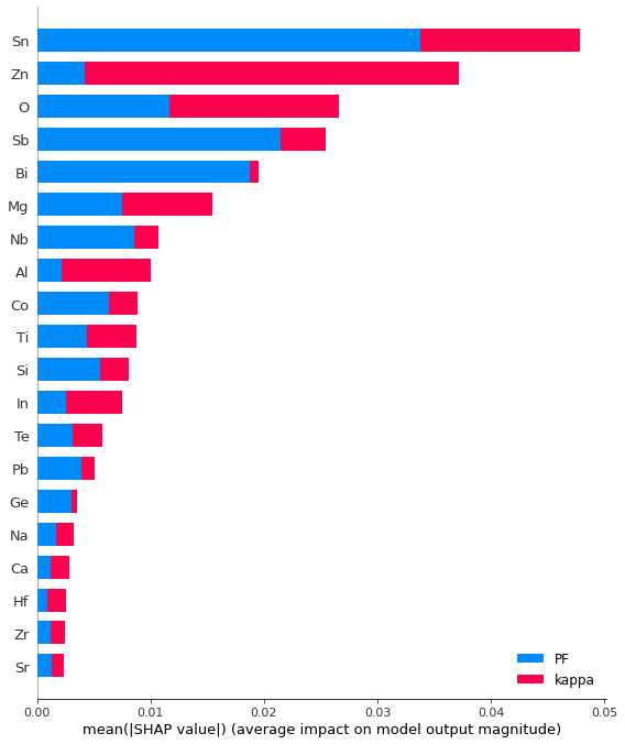

The bars' width implies the extent (magnitude) of the impact of features on the targets and displays absolute values. For instance, Zn displays a wider red bar than a blue bar, indicating it plays a stronger role in terms of thermal conductivity than PF.

However, to understand the nature of the contribution of features on the final target, we need a summary plot for a single target illustrating both the intensity and direction of impact, i.e. whether the feature is favorably or adversely affecting the said target. Let me illustrate this point.

Reading Single Target Summary Plot

Here are the plots showing the influence of features (elements) on kappa and PF, taken individually.

Index 0 represents kappa

shap.summary_plot(shap_values_rf[0], X_train)

Index 1 represents PF

shap.summary_plot(shap_values_rf[1], X_train)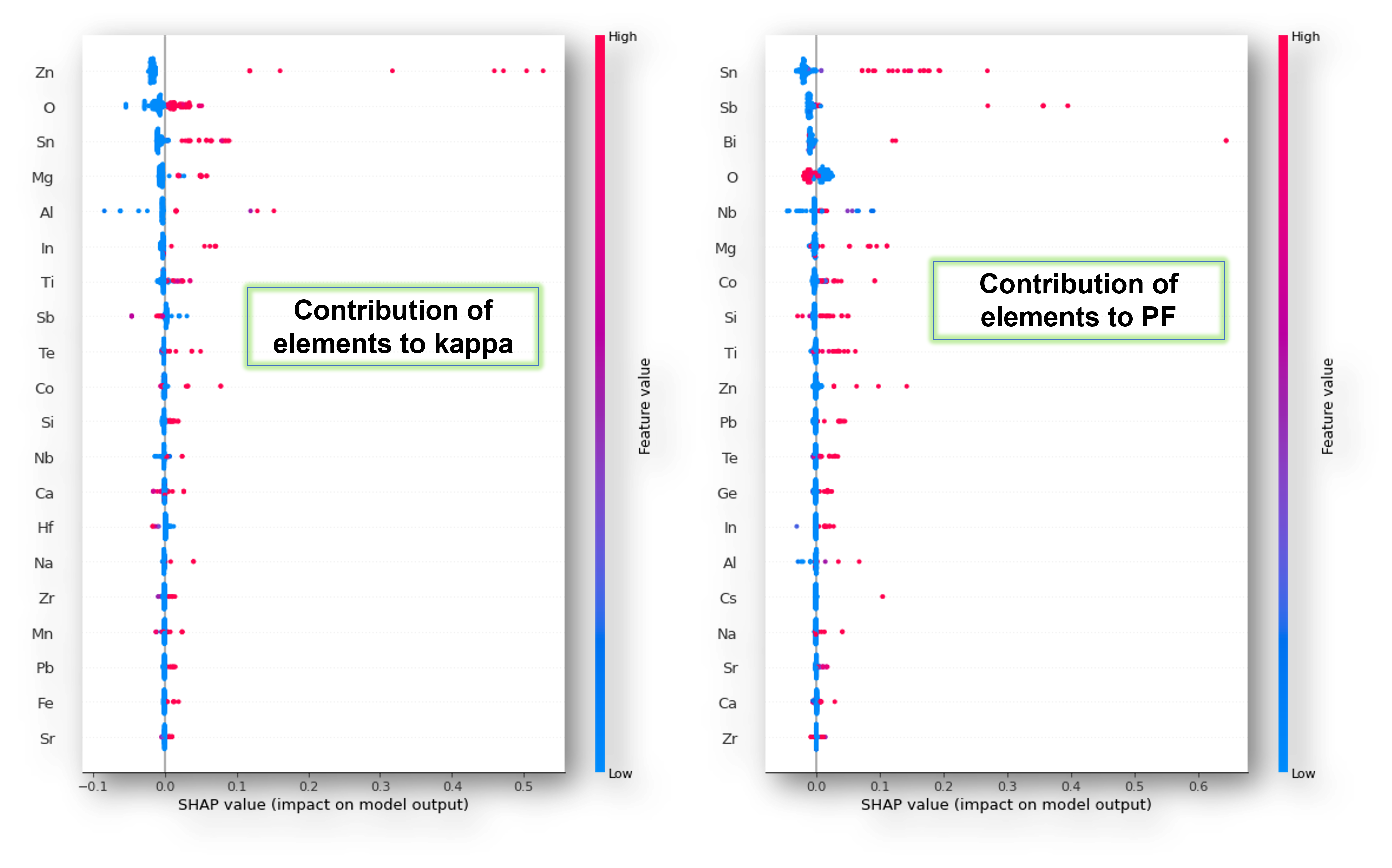

The strength of contributions is color-coded red and blue where, red is strong, and blue is weak. Plus, the sign of SHAP values of a feature tells whether it has a positive or negative impact on the target.

For example

Zn has more positive correlations with kappa than that with PF.

Sb has a high positive correlation with PF and a high negative correlation with kappa.

Thus, SHAP summary plots help select elements that can enhance PF and decrease kappa-a combination for an ideal thermoelectric composition.

Note: If you choose to apply an artificial neural network (ANN) for fitting the dataset and building an appropriate model, a KernelExplainer function should be used for the SHAP analysis.

Click to avail the entire code.

SHAP Analysis for Multiple Targets in Machine Learning